Feed-forward Neural Network Based Transient Stability Assessment of. 132KV Sub-transmission Power System Network: Case Study Afam to. Port-Harcourt ...
International Research Journal of Engineering and Technology (IRJET)
e-ISSN: 2395-0056
Volume: 05 Issue: 03 | Mar-2018
p-ISSN: 2395-0072
www.irjet.net
Feed-forward Neural Network Based Transient Stability Assessment of 132KV Sub-transmission Power System Network: Case Study Afam to Port-Harcourt Town (Z4), Nigeria Tekena K. Bala1, Chinweike I. Amesi2, Samuel N. Ndubisi3 1Electrical
Engineering Department, Rivers State University, Nkpolu, Port-Harcourt, Nigeria Engineering Department, University of Port-Harcourt, Nigeria 3Professor, Electrical/Electronic Engineering Department, University of Port-Harcourt, Nigeria ---------------------------------------------------------------------***--------------------------------------------------------------------2Electrical/Electronic
synchronous generators are cascaded to generate electric power for man’s needs. Usually, in a power generating station two or more generators are synchronism to provide bulk electric power through transmission networks.
Abstract - The adverse effects due to disturbance
especially three-phase fault on power system networks are severe; therefore, it is pertinent to determine the characteristics behavior of these networks when a fault occurs and to maintain or avoid the impact of these disturbances on the power system networks. This research work is geared towards evaluating the critical clearing time and the rotor angle by which the circuit breaker(s) are /is required to open during abnormal condition without damage to generators under synchronism, etc. The objectives of the research work were achieved in threefold: Firstly the test system 132KV sub-transmission network was modeled using ETAP 7.0 Software to perform the time domain simulation processes and obtained results for further analysis. Secondly, in MATLAB environment, programs using Runge-Kutta (order-2) method was also used to solve the swing equation of SEMIB for further data collection. Thirdly, selected features from Runge-Kutta’s method’s results were now fed into the feed-forward neural network (FFNN), as inputs and targets/outputs to map out the CCT required for the operation of the circuit breakers. Thus, from the comparative results of the (FFNN) and the conventional (R-K) method shows that both can be complementary to evaluate the CCT and rotor angle for transient stability assessment of power system networks.
The effect and performance of these synchronous machines after been disturbed is very important in the stability of the power system. It is noted that in power system stability studies especially the transient events: the rotor angle, power transfer capabilities, frequency, and voltage, etc., are fundamental electrical variables one need to check. Rotor-angle stability problem is a function of ‘transient stability’ and ‘small-disturbance stability’ problem linked with the operation of synchronous machines being in parallel through long-distance transmission lines delivery bulk electric power. From a visual point of view, transient stability is a function of abnormality in power system that required immediate normalcy. That is the ability of an electric power system to keep its synchronous machines’ in synchronized operation when subjected to large or small disturbance. It is also a nonlinear, high-dimensional problem from the theoretical point of view of power system stability analysis as seen in [1]. In this article, we shall utilize the advantages of applying feed-forward neural network, a class of ANN in assessing the critical clearing time of appropriate circuit breaker in connection to generators lumped as Single Machine connected to Infinite Bus System as the main aim.
Key Words: Critical clearing time, ETAP software, MATLAB, FFNN, Power system networks, Transient stability, Torque angle, etc.
1. INTRODUCTION
1.1 Statement of Problem
The increasing demand and needs for electric power, networking and consumption on daily basis are neverending. Currently, in all sectors of life enterprise, electric power is ultimate. The networks in which electric power is been transported are very /extremely complex; bulk electric power is transmitted over the interconnected network of transmission lines linking generators, power transformers, loads, etc., to give man’s comfort. Successful operation of a power system depends largely on the ability to readily provide reliable and uninterrupted service delivery to the loads. Constant voltage and frequency at all times are required by consumer’s equipment (loads) to operate satisfactorily. High powered turbines and
© 2018, IRJET
|
Impact Factor value: 6.171
Disturbances such as switching OFF and ON of power circuit, short circuit fault from power system network, loss of synchronous generators, surges due to lightning effect, etc. had the consequences of losing stability following or after the occurrence of a disturbance on power system network. The factor of an unintentional power outage is a problem. Sometimes the disturbance on the network may be small or large depending on the nature and location of the disturbances.
|
ISO 9001:2008 Certified Journal
|
Page 707
International Research Journal of Engineering and Technology (IRJET)
e-ISSN: 2395-0056
Volume: 05 Issue: 03 | Mar-2018
p-ISSN: 2395-0072
www.irjet.net
fault location, the AVR’s response time is too large to respond to such an event resulted from either loss of loads, transmission network collapse from a three-phase faults, etc.,[2].
1.2 Objectives of Assessment a)
Is to determine the characteristic behavior of the system network when subjected to a three-phase fault.
b)
Is to evaluate, and predict the status of the network in regards to the critical clearing time (CCT) of the circuit breakers and to classify the network whether transiently it is stable or unstable.
c)
To assess the active power transfer of the power system network due to a transient event at various fault location that may affect the performance, reliability, and stability of operation.
The researchers Kothari and Nagrath, in their book mentioned (Kundur P. et al., vol. 19, no.2, May 2004), an IEEE transaction on power system; defined Power system stability as: “the capability of an electric power system with known initial operating condition, to recover a state of operating balance after being subjected to a physical disturbance, with most system variables restrained in such a way that, practically the whole system remains intact” [3]. Of course, the nature of a system should either be stable or unstable; in electric power systems and networks, the unstable power system may cause blackout otherwise unintentional power outage within the area under consideration. However, to provide a secure and a stable electric power through the network(s) that must be reliable, safe, etc., one needs to assess the transient stability level of the network fast and accurately.
[
1.3 Scope of Assessment The total assessment of all 132kV, 33kV, 11kV utility networks in Rivers state will pose a huge stress in the assessment processes; hence we shall focus on the following area as a case study: i)
The 132kV network emanating from Afam to PortHarcourt (PH) Town (Zone4) at Amadi junction and some distribution network in their load terms.
ii)
Determination of the critical clearing time for the appropriate circuit breakers installed at the generator ends and the torque angle, voltage profile, and power transfer capability between generation and loads.
According to (Karami, 2011), determination of transient stability of power system one has to resort using the most frequently used technique (time domain simulation technique) to evaluate the given set of nonlinear equations that describe the dynamic system equations. In reality, the condition of loading of the power system and the system parameters of the state actually varies from those presumed at the preliminary planning stage [4].
2.2 Application of Machine Learning Approaches in Electric Power Systems and Networks, etc.
2. LITERATURE REVIEW
The growing trend of machine learning approaches such as ANN, AI, expert systems, fuzzy logic, etc., to electric power systems studies, etc., are presented in the various literature. As seen in (Orike, 2015) that computational intelligence (CIs) are now complementary the assessment of those critical areas in electric power systems and networks to quickly achieve the desired results. These areas are transient stability assessment; static and dynamic security assessment; identification, modeling and prediction/evaluation; control; maintenance analysis; load forecasting; fault location and analysis [5].
2.1 Time Domain Simulation in Power System The behaviors of synchronous machines following or after a small or large disturbance on the interconnection of generators, transformers, power transmission networks and load are very much vital as stated earlier. In the yesteryears, due to the rigorous circumstances involving the analysis of transient stability in electric power system and networks, in literature, the use of ‘time-domain’ methods (i.e. numerical integration) was in used before the arrival of numerical computers; system motion equations were carried out manually to determine the machines’ swing curves. Thus, the evolution of ‘rotor angle’ with time was far noted, in Park and Bancker, 1929 as referenced in [1].
2.2.1 Neural Networks in Electric Power Systems The increasing nature of interconnection of power systems and its complexity has a resort to new approaches to assess the status. As seen in (Pothamsetty et al., 2014) in their paper: “power system transient stability margin estimation using artificial neural networks,” presented multi-layered perceptron (MLP), a neural network used to approximate the normalized transient stability sideline. The MLP neural network was structured to map the nonlinear relationship between the initial operating state and normalized transient stability sideline. In their works, time domain
The sudden occurrence of transient impact on power systems network is totally inevitable rather it is better we geared towards minimizing it. In fact, there are cases where national grid network collapses thereby rendering zero power to consumers. According to Epili and Vadirajacharya, the duration of time for the occurrence of this transient is very short, even the generators close to
© 2018, IRJET
|
Impact Factor value: 6.171
|
ISO 9001:2008 Certified Journal
|
Page 708
International Research Journal of Engineering and Technology (IRJET)
e-ISSN: 2395-0056
Volume: 05 Issue: 03 | Mar-2018
p-ISSN: 2395-0072
www.irjet.net
simulation method together with potential energy margin surface method was used to acquire the training set of NN.
2.2.3 Power System Networks Performance In terms of power systems networks analysis (Ebrahimpour, et al., (n.d)) introduces a new model of the neural network in their research work for estimation of transient stability named committee neural network (CNN). In their paper, a mixture of the experts (ME) was used to assess the transient stability of power system after faults occur on transmission lines, in a way that, the problem space was distributed into some subspaces for the experts, and then the outputs of experts are joined by a gating network to form the final output. Using the IEEE 9bus and IEEE 14-bus as a test sample, the simulations were made with an injection of three-phase faults on the test systems. In addition, input data required for further analysis from the time domain simulation were feds into the mixture of an expert system for proper classification of the systems’ status - whether the system is stable or unstable [12].
It is worthwhile to note that, the worst contingency expected is best simulated in advances as to curtail the status of the scenario and to take advantage of a preventive control rather than total failure in due course. The application of the time-domain simulation (TDS) method for on-line or off-line analysis is the very best; accurate for determining the transient stability problem. Due to circuit modeling conditions, a method known as Equal Area Criterion is limited in its application. Large power system now utilizes neural network in assessing transient stability [6]. Also, Bourguet and Antsaklis (1994), presented ANN application in the electric power industry, a technical report which highlighted - power plants and control problems, using neural networks, a perspective of power systems such as security system, load predicting, and fault analysis [7].
2.2.4 Fault Location and Assessment
In (Abdul Wahab et al., 2007), probabilistic neural network (PNN) and least squares support vector machine (LS-SVM) methods were applied to assess the transient stability of the IEEE 9-bus network; a test system for the verification of the methods. Prior to the implementation of the PNN and LS-SVM, time domain simulations were carried out for the purposes of obtaining selected training data sets while considering several contingencies. As stated in their works, simulations were done using the MATLAB-based PSAT. And that, time domain simulation method was chosen to assess the transient stability of the power system because it is the most accurate method compared to the direct method [8]. Again, in the article [9], ANN was used. The critical fault clearing time obtained via multilayer feedforward artificial neural network was compared to the results of the conventional equal area criterion method.
One of the major causes of a power outage is the failure of electrical equipment. For reliability, security, and availability of power, it is required to have good detection, fault location point and diagnosis systems in the power system operation. ANNs are being studied as classifiers of failures in electrical apparatus, and successful results have been recorded. The development of ANN gives the extra advantage of recording the failures and can also reproduce them [13]. In (Olulope et al., 2010), the application of time domain integration schemes was first utilized; then, multi-layered feedforward network (a class of artificial neural networks) trained with Levenberg Marquardt (LM) back propagation algorithm was used for estimating the critical fault clearing time (CCT) of a power system. In their research work, a single disturbance such as three-phase fault was injected into the test network. From the TDS output, selected known features were taken as inputs and the critical fault clearing time (CCT) estimated previously as the desired target. Using single machine infinite bus system (SMIB) model; their test system was modeled using DIgSILENT software packages.
2.2.2 Static and Dynamic Security Assessment On this subheading, the utilization of expert systems, decision trees, etc. was also mentioned in (Kalyani and Shanti Swarup, 2009). Some prototypes of neural networks were studied as classifier design. In their assessment, features collections were made using a forward sequential technique. On the online security assessment, suitable classifier design in pattern recognition with input features classification was made to assess the system security profile as stated in [10].
It was noted that there are two principal methods of assessing transient stability: evaluation and prediction method. In the analysis of power system stability, the critical fault clearing time must be evaluated; while prediction of the power system conditions states whether it is stable or unstable gives the classification criterion, thus, the critical clearing time is insignificant when considering stability prediction [14].
In (Sobajic and Pao, 1989) presented a key-work of the use of artificial neural networks (ANN) in electric power systems. An adaptive pattern recognition approach based on a Rumelhart feed-forward neural network with a backpropagation learning scheme was applied to synthesize the critical clearing time (CCT). A parameter that is paramount in the post-fault dynamic analysis of interconnected systems [11].
© 2018, IRJET
|
Impact Factor value: 6.171
With reference to (Amjady and Majedi, 2007), assessment of CCT for a power system, radial basis function networks can also perform the task. In their work, critical clearing
|
ISO 9001:2008 Certified Journal
|
Page 709
International Research Journal of Engineering and Technology (IRJET)
e-ISSN: 2395-0056
Volume: 05 Issue: 03 | Mar-2018
p-ISSN: 2395-0072
www.irjet.net GH = K.E = ½ M s
time was defined as: If the fault is cleared after its occurrence as soon as possible in power system, that immediate maximum time it takes to cleared the fault to keep the system transiently stable is called the Critical Clearing time (CCT) [15].
MJ
-- (1.4)
MJ-s/elect.rad MJ-s/elect..rad
-- (1.5)
MJ-s/elect. degree
-- (1.6)
3. METHODOLOGY 3.1 Methods Applied to Transient Stability Studies
Substituting equation (1.5) or (1.6) into equation (1.3) the swing equation becomes
In literature, there are different methods used in the study of transient stability assessment, but few methods will be mention here:
-- (1.7) Dividing by equation (1.7) by Gbase (base MVA) rating of the machine(s), we have:
(a) Time domain simulation of the power system network (b) The step-by-step method of numerical solution of swing equation
(
)
) Pu
(
-- (1.8)
(c) A digital solution of swing equation using Runge-Kutta methods
-- (1.9)
(d) Equal-area criterion
But, if Grated = Gbase, then, we have
(e) Liapunov’s direct method, (f) Machine learning approaches, etc., [3], [5].
-- (2.0)
From the above mentioned techniques, we will utilize the techniques of (a),(c), (d) and (f) to a model of Single Equivalent Machine connected to the infinite bus system (SEMIB) to demonstrate the electromechanical angular and voltage swings when a three-phase fault occurs on one of the double circuit sub-transmission lines. The threephase balance fault will be injected into the line at different location or point on the line. The test network will be modelled and simulated using ETAP software as the simulation tool.
Equation (1.9) is the per-unit swing equation. We shall use the per-unit values in our computation in the digital solution of solving the swing equation using Runge-Kutta (order-2) method [3], [18].
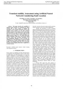
3.3 The Test System Network The modelled diagram of the positive sequence reactance network was further reduced to Fig.1.
3.2 The Swing Equation
Afam Eq.Gen. (IV &V) Eg'=1.75pu
-- (1.1)
G a.
MW or pu
-- (1.2)
j0.306pu Afam-PH Bus
-- (1.3)
CB6
L2 j0.081pu
L1 j0.081pu
Equation (1.1) or (1.3) is the swing equation describing the motion of the generator.
CB8
Let Gbase = base MVA
CB9
PH(Z4) Bus b
Grated = machine rating in MVA (3-ph)
Fig.1: Single Equivalent Machine Connected to Infinite Bus bar (SEMIB)
M = moment of inertia of the generator
Impact Factor value: 6.171
0
Infinite Bus
f = power supply frequency in Hertz (HZ) or cycle per second
|
j 0.0717pu 1
H = inertia constant in MJ/MVA or MW-s/MVA
© 2018, IRJET
CB7
|
ISO 9001:2008 Certified Journal
|
Page 710
International Research Journal of Engineering and Technology (IRJET)
e-ISSN: 2395-0056
Volume: 05 Issue: 03 | Mar-2018
p-ISSN: 2395-0072
www.irjet.net
3.4 Terms of Some Parameters and Computation Let = voltage (emf) behind transient reactance; = active power transferred to the system; Pm = mechanical power input to the rotor shaft; Pa = accelerating power; V= the voltage at infinite bus bar; Pmaxbf = maximum power that can be transferred before fault; Pmaxdf = maximum power that can be transferred during fault; Pmaxaf = maximum power that can be transferred after isolation (i.e. clearance) of fault, Xbf = transfer reactance of the entire network before –fault; Xd = steady – state synchronous reactance of the generator; Xd = direct- axis transient reactance of the generator; Xd= subtransient reactance of the generator; XL = transmission lines reactance (neglecting Ro).etc., [3],[18].
Transfer reactance of the entire network before-fault condition (
)
For active power transferred before-fault condition
:
Initial power angle is given by
Under transient condition Xd Xd ˂ Xd and Xd ˂ Xd ˂ Xd During transient condition Xequ = Xd + XL |
-- (2.1)
|| |
pu
-- (2.2)
For active power transferred during fault condition, @ 0.00 s to 0.150 s fault clearing time setting, when δ=66.94 deg.
3.5 Critical Clearing Angle (δcrang) For any given initial load there is a critical clearing angle and if actual clearing angle exceeds critical clearing angle the system becomes unstable otherwise it will be stable. Equal-area criterion is basically suitable for one machine system with infinite bus-bar but with a limitation – it is not feasible to evaluate the critical clearing time, CCT required to set the circuit breakers rather the maximum torque angle and critical clearing angle can be evaluated. Thus, using the equal-area criterion for critical clearing angle, δcrang, we have (
(
)
For active power transferred after-fault condition, :@ 0.00 s. to 0.151s fault clearing time setting, when δ=67.08 deg. (
)
Maximum torque angle,
) elect. deg.
Where:
is given by ,
from equation (2.6)
above; and
-- (2.3)
⁄
-- (2.4) -- (2.5)
Maximum torque angle,
is given by elect.deg.
Using the equal-area criterion for critical clearing angle, δcrang, we get
-- (2.6)
Case 1: On 10% Fault Location on Line 1 (i.e. 3.835 KM) from Afam 132KV bus to PH (Z4) 132KV line Using Fig. 1 shown above and the data from the load flow simulation report, we have
© 2018, IRJET
|
Impact Factor value: 6.171
|
ISO 9001:2008 Certified Journal
|
Page 711
International Research Journal of Engineering and Technology (IRJET)
e-ISSN: 2395-0056
Volume: 05 Issue: 03 | Mar-2018
p-ISSN: 2395-0072
www.irjet.net
In order to achieve the numerous computation involved in the analysis, A Program for the transient stability of single machine connected to the infinite bus using Runge-Kutta (Order-2) method of solving swing equation was implemented in MATLAB R2013a environment [17].
equivalent machine under consideration and is kept constant, delta (δ) is the rotor angle during fault condition, (Pmaxdf) is the maximum electrical power delivered during fault condition, (Pe2) is the real power delivered during fault condition, and (ω) is the rotor angular speed. Levenberg Marquardt (LM) back-propagation algorithm will be used to train the network in the multilayered feedforward neural network to evaluate the critical clearing time (CCT) [5], [9].
3.6 Simulation of the Test System Network Electrical Transient Analyzer Program (ETAP) is powerful simulation software [16] used to model power system networks and carry out the simulation. In the first scenarios, the load flow results are obtained on 100 MVA base systems. We will inject three phase balance fault at different point/location on the line in order to ascertain the true state of the line under fault condition and to evaluate for setting of the circuit breakers critical opening time at different faults point say 10%, 20%, 30%, 40%, 50%,…..100% of 38.35KM on line1 from Afam bus to Port Harcourt Town (Zone 4). The operating voltage is 132kV. From the load flow and transient stability assessment (ETAP simulation report) certain generated data were collected for further analysis using Equal Area Criterion (EAC) and Runge-Kutta's (Order-2) method of numerical analysis using MATLAB R2013a software.
b) The second section is responsible for applying the concepts of the FFNN (expert system) to solve the transient stability problem using the data supplied from the first section. Here, some percentage of the inputs data are used as a train set, test set; and validation of the network configuration. The performance of the model is a function of certain classification accuracy and misclassification function. The training of the inputs data sets takes more time as the case may be. In this research work, the data sets for 10%, to 50% faults location on line 1 utilizes 10,20,10 neutrons while the data sets for 60% to 100% faults location inputs data utilized 20,10, 20 neutrons in the hidden layer of the FFNN during the training as configured. c) There should be some form of conformity between the ‘targets’ value used and the real ‘output’ from the trained network, to actualize better network plots. The FFNN is capable of evaluating the critical faults clearing time (CCT) of the power system network as the desired output y. The results may be compared with the conventional results. After simulation of the input-trained data sets with equal respective targets, the regression plots and performance plots are checked to for best plots. Thereafter, a new set of the inputs data are fed into a saved M-file to generate a corresponding output as desired. The regression plots and performance plots are very important; it indicates the perfection of the trained data set and the target/ output. See the various figures/plots below.
3.7 Utilization of Runge-Kutta (Order-2) method to the various cases: For 10% Fault Location (3.835KM) on line 1 Input data into the program for 10% of Line1: Pm = 3.8100 pu; deg = 1.1489 radian; Pmaxbf = 4.1750 pu; Pmaxdf = 3.2270 pu; Pmaxaf = 4.2230 pu; H = 14.6500 MW-s/MVA; Fault clearing time (FCT setting): 0.00 – 0.150 s; Total simulation time used: 1.0 sec. After the first computation and yielding the desired results, we now replace the data in the input section of the program with new sets of data, simulate again for all percentage stated. The critical clearing time is realized during the simulation by trial and errors. Thereafter, selected features from the program results were fed into the feed-forward neural network to further estimate the desired CCT.
3.9 Some Neural Network Classifier The neural network has the ability to simulate large or small data without misplacing the uniqueness of the dynamic behaviour of that system. All are classifiers of artificial neural network used nowadays in the assessment of power systems/networks:(i) Multilayer Perceptron (MLP) Neural Network; (ii) Learning Vector Quantization (LVQ) Neural Network; (iii) Probabilistic Neural Network (PNN); (iv) Adaptive Resonance Theory Mapping (ARTMAP), (v) Mixture of Experts system, etc. The neural networks models are designed with respective train algorithm [10], [11], [12].
3.8 Utilization of the (FFNN) to Evaluate the CCT The utilization task is in three sections: a) This first section is responsible for acquiring the training data set in order to train the multi-layered feedforward neural network (FFNN) and allow it to adjust its parameters to form a configuration that links the inputs with the outputs. Here, the training data sets are output results of the solution of Runge-Kutta method of solving the swing equation. The training of the FFNN will utilize selected features as input (M; δ; Pmaxdf; Pe2; ω), (refer to equation 2.7, below) and the critical fault clearing time (CCT), (refer to equation 2.9, below) as desired target/output. Where M is the moment of inertia of the
© 2018, IRJET
|
Impact Factor value: 6.171
A Multi-layered Perceptron (MLP) model is a feedforward neural network model capable of mapping given input data sets with the corresponding target to produce
|
ISO 9001:2008 Certified Journal
|
Page 712
International Research Journal of Engineering and Technology (IRJET)
e-ISSN: 2395-0056
Volume: 05 Issue: 03 | Mar-2018
p-ISSN: 2395-0072
www.irjet.net
an output. The network in its training period of the data sets given, establishes input-output relationships.It consists of input, two or more layer of neurons (called the hidden layers) with nonlinear activation or transfer functions (tan-sigmoid transfer function) and an output layer (linear transfer function) often time. The network can be trained with Levenberg-Marquardt (LM) backpropagation algorithm [10], [11], [12].
+1
0 -1
3.9.1 Transfer Function/Activation Function
y = Purelin (n) Fig. 3: Linear Transfer Function Adapted from: Mathworks
The transfer function controls the amplitude of the output by translating the output of the neuron to its input before finally outputting the result. There are lots of transfer functions available in the neural network toolbox programs [17]. However, transfer functions frequently used for multilayer feed-forward neural network are: 1)
3.9.2 The Feed-forward Neural Network in MATLAB Environment Using Multilayer feed-forward neural network, we can increase the hidden layer from the ‘default’ to any desired hidden layers [17]. From the network below, we have three (3) hidden layers; the hidden size, each has 20, 10 and 20 neurons in parenthesis- square bracket upon round bracket. Fig. 4 shows the screenshot architecture of the multilayered feed-forward neural network utilized in this research work.
Tan-sigmoid Transfer Function (Tansig): Sigmoid output neurons are applied for pattern recognition problems. Linear output neurons are applied for function fitting problems. Fig.2 shows the tan-sigmoid transfer function [17].
2)
Linear Transfer Function (Purelin): In these types of functions the neurons are applied in the final layer of the multi-layered network as function approximations. Fig.3 shows the linear transfer function applied in multilayer networks with backpropagation training algorithms [17].
3)
Log-sigmoid Transfer Function (Logsig): This transfer function collects the input variable of any value between plus (+) and minus (–) infinity and compresses the output into series of 0 to 1 [17]. Fig 4: Screenshot of Multilayered Feed-forward Neural Network (FFNN)
+1
α 0
n
Sample Call-Out Program for the FFNN in MATLAB Environment
n
Inputdata= […]; Targetdata= […];
-1
net=feedforwardnet ([hiddensize1,hiddensize2,..hiddensizen],'trainlm');
α = tansig(n) Fig 2: Tan-Sigmoid Transfer Function Adapted from: Mathworks
net=configure(net,Inputdata,Targetdata);view(net); net=init(net); net=train(net,Inputdata,Targetdata) Output ofTarget = net (Inputdata) perf = perform(net,Inputdata,Targetdata) Input data set:
© 2018, IRJET
|
Impact Factor value: 6.171
|
ISO 9001:2008 Certified Journal
|
Page 713
International Research Journal of Engineering and Technology (IRJET)
e-ISSN: 2395-0056
Volume: 05 Issue: 03 | Mar-2018
p-ISSN: 2395-0072
www.irjet.net
Inputs =
chart presentation of the FFNN versus numerical (R-K) method for CCT determination.
-- (2.7) [
Table I Results of the Time Domain Simulation (TDS) using ETAP Software
]
[
]
Perce ntage Fault Locati on
-- (2.8)
If R = m, S = n, for (m n) matrix,
Three phase Fault Location From Afam bus to PH(Z 4)Bus (KM) 3.835
Equivale nt Inertia Constant H (MJ/MVA ) 14.65
Pmaxdf (During fault)
Pe2 (Durin g fault)
(Pu)
(Pu)
3.0111
2.9700
67.1
0.37
20
7.67
14.65
3.1444
3.1200
66.7
0.55
30 40
11.505 15.34
14.65 14.65
3.2417 3.3126
3.2300 3.3100
69.1 68.5
0.56 0.56
50 60
19.175 23.01
14.65 14.65
3.3809 3.4249
3.3800 3.4200
68.2 66.6
0.56 0.56
70
26.845
14.65
3.4627
3.4500
66.7
0.56
80 90
30.68 34.515
14.65 14.65
3.3927 3.5244
3.3800 3.4900
66.7 66.6
0.56 0.56
100
38.35
14.65
3.5252
3.4900
66.6
0.56
(%) 10
Where M = moment of inertia of the equivalent generator in Pu; δn=rotor angles during a respective fault condition in radian; Pmaxdf = Maximum power delivered during a fault condition in Pu; Pe2 = Real power delivered during a fault condition in Pu; ωn.= Rotor angular speed in Pu. Target data ] -- (2.9) Where n = no. of cct corresponding to a set of input data.
4.1. Results From the different stages of assessment of the 132KV power system network- (a case study of Afam to PortHarcourt (PH) Town (Zone4)) operating at 132KV (incomer) and 33KV (out-going). Table I shows the results of the respective percentage fault location of line 1 during the time domain simulation (TDS) of the transient stability assessment using ETAP Software; the base case analysis.
t
di
0 0.0500 0.1000 0.1500 0.2000 0.2500 0.3000 0.3500 0.4000 0.4500 0.5000
1.1490 1.1606 1.1952 1.2517 1.3283 1.4231 1.5346 1.6618 1.8049 1.9660 2.1492
t 0 0.0500 0.1000 0.1500 0.2000 0.2500 0.3000 0.3500 0.4000 0.4500 0.5000
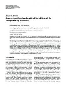
Fig. 6 presents a graph of maximum power delivered (Pmax) versus CCTs (from Table III.); Fig. 7 shows the graph of real power delivered during fault conditions (Pe2) versus CCTs (from Table III) while Fig. 8 is the graph of critical clearing angle (δcrang) versus CCTs (from Table IV). Fig.9 is the regression plots for (10%-100%) fault location and Fig. 10 the performance plot for (10%100%) fault location using the FFNN. The column chart for CCT versus 10%-100% fault location using FFNN is shown in Fig.11.
(s)
wi
Pm
0 0.4642 0.9125 1.3320 1.7156 2.0641 2.3869 2.7030 3.0412 3.4410 3.9558
3.8100 3.8100 3.8100 3.8100 3.8100 3.8100 3.8100 3.8100 3.8100 3.8100 3.8100
Pmaxdf k1 4.1750 3.2270 3.2270 3.2270 3.2270 3.2270 3.2270 3.2270 3.2270 3.2270 3.2270
l1
0 0 0.0232 0.0456 0.0666 0.0858 0.1032 0.1193 0.1352 0.1521 0.1721
k2
0 0 0.4642 0.0232 0.4561 0.0460 0.4331 0.0673 0.3999 0.0866 0.3632 0.1039 0.3314 0.1198 0.3137 0.1350 0.3197 0.1511 0.3598 0.1700 0.4459 0.1943
l2
ddi
0 0.4642 0.4405 0.4059 0.3674 0.3338 0.3143 0.3185 0.3566 0.4400 0.5835
0 0 0 0.0116 0.4642 66.4977 0.0346 0.4483 68.4808 0.0565 0.4195 71.7152 0.0766 0.3837 76.1038 0.0949 0.3485 81.5389 0.1115 0.3228 87.9268 0.1272 0.3161 95.2141 0.1431 0.3382 103.4157 0.1611 0.3999 112.6433 0.1832 0.5147 123.1399
dwi
d(i+1)
di
wi
Pm
1.1490 1.1606 1.1952 1.2517 1.3283 1.4231 1.5346 1.6618 1.8049 1.9660 2.1492
0 0.4642 0.9125 1.3320 1.7156 2.0641 2.3869 2.7030 3.0412 3.4410 3.9558
Pmaxbf k1
3.8100 3.8100 3.8100 3.8100 3.8100 3.8100 3.8100 3.8100 3.8100 3.8100 3.8100
4.1750 4.2230 4.2230 4.2230 4.2230 4.2230 4.2230 4.2230 4.2230 4.2230 4.2230
l1
k2
l2
0 0 0 0 0 0.4642 0.0232 0.4642 0.0232 0.4561 0.0460 0.4405 0.0456 -0.0636 0.0424 -0.0993 0.0416 -0.0981 0.0366 -0.1269 0.0359 -0.1253 0.0297 -0.1473 0.0291 -0.1455 0.0218 -0.1615 0.0214 -0.1596 0.0135 -0.1704 0.0132 -0.1684 0.0048 -0.1747 0.0046 -0.1727 -0.0040 -0.1749 -0.0041 -0.1729 -0.0127 -0.1709
ddi
dwi
d(i+1)
0 0.0116 0.0346 0.0440 0.0391 0.0328 0.0255 0.0174 0.0090 0.0003 -0.0084
0 0 0.4642 66.4977 0.4483 68.4808 -0.0814 71.0037 -0.1125 73.2438 -0.1363 75.1227 -0.1535 76.5822 -0.1650 77.5817 -0.1716 78.0958 -0.1738 78.1124 -0.1719 77.6309
Table II(c) Critical Clearing time found after 0.15s for 10% Fault Location (Critically stable) t
di
0 1.1490 0.0500 1.1606 0.1000 1.1952 0.1500 1.2392 0.2000 1.2783 0.2500 1.3111 0.3000 1.3366 0.3500 1.3541 0.4000 1.3630 0.4500 1.3633 0.5000 1.3549
The comparative presentation of the results of the (FFNN) and the conventional method (Runge-Kutta order2) is shown in Table IV whereas Fig.12 shows the column
Impact Factor value: 6.171
(deg.)
Table II (b) Fault Cleared at 0.15s for 10% Fault location (Stable)
Table II (a), (b) and (c) are results of the application of Runge-Kutta method solution of the swing equation with unstable, stable and critically stable conditions for only 10% fault location on (line 1) whereas Table III is the summary results (all percentage) using Runge-Kutta method. Fig 5 shows the graph of the swing curve for 10% fault location on line1 with (sustained fault, fault cleared curve and critically stable curve).
|
Critical Clearin g Time (CCT)
Table II (a) Sustained Fault for 10% Fault Location (Unstable)
4. RESULTS AND DISCUSSION
© 2018, IRJET
Critical Clearing Angle, dcrang
|
wi
Pm
Pmaxdf
0 3.8100 4.1750 0.4642 3.8100 3.2270 0.9125 3.8100 3.2270 0.8310 3.8100 3.2270 0.7185 3.8100 3.2270 0.5822 3.8100 3.2270 0.4287 3.8100 4.2230 0.2637 3.8100 4.2230 0.0921 3.8100 4.2230 -0.0816 3.8100 4.2230 -0.2535 3.8100 4.2230
k1
l1
k2
l2
ddi
dwi
d(i+1)
0 0 0 0 0 0 0 0.4642 0.0232 0.4642 0.0116 0.0232 0.4561 0.0460 0.4405 0.0346 0.0456 0.4331 0.0673 0.4059 0.0565 0.0666 0.3999 0.0866 0.3674 0.0766 0.0858 0.3632 0.1039 0.3338 0.0949 0.1032 -0.1968 0.0934 -0.2192 0.0983 0.0928 -0.2187 0.0819 -0.2193 0.0873 0.0819 -0.2198 0.0709 -0.2052 0.0764 0.0712 -0.2066 0.0609 -0.1826 0.0661 0.0615 -0.1847 0.0523 -0.1555 0.0569
ISO 9001:2008 Certified Journal
|
0 0.4642 0.4483 0.4195 0.3837 0.3485 -0.2080 -0.2190 -0.2125 -0.1946 -0.1701
66.4977 68.4808 71.7152 76.1038 81.5389 87.1703 92.1745 96.5498 100.3352 103.5946
Page 714
International Research Journal of Engineering and Technology (IRJET)
e-ISSN: 2395-0056
Volume: 05 Issue: 03 | Mar-2018
p-ISSN: 2395-0072
www.irjet.net
Output Result for 10% Fault Location δmax = 114.1671 deg (maximum angle); δcrang = 80.5192 deg. (critical clearing angle), Power delivered during fault condition, Pe2 = 2.9700 pu; Pmax = 3.0111 pu (maximum power delivered at δcrang)
Critical Clearing angle during fault condition in deg.
plot of dcrang verus cct
Generator swing curve 130
Sustained fault (Unstable) @0.15 sec
110
Critically stable curve@ 0.27 sec
100
98 96 94 FFNN
92 Runge-Kutta
90 88 86 84 82 80 0.25
90
0.3
0.4
0.45 0.5 0.55 Critical Clearing Time in s.
0.6
0.65
0.7
0.75
0
0.05
0.1
0.15
0.2 0.25 0.3 Time t in seconds
0.35
0.4
0.45
0.5
Training: R=1
Fig 5: Graph of Swing Curves for 10% Fault Location on Line1 (Sustained Fault, Fault Cleared and Critically Stable Curve) plot of Pmax verus cct 3.7
0.7 0.65 0.6 0.55 0.5 0.45 0.4 0.35 0.3 0.3
0.4
0.5
0.6
0.7
Data Fit Y=T
0.65 0.6 0.55 0.5 0.45 0.4 0.35 0.3
0.7
0.3
0.4
0.5
Target
3.6
Output ~= 1.1*Target + -0.059
3.4
3.3
3.2
3.1
0.7
0.6 0.55 0.5 0.45 0.4 0.35 0.3 0.3
0.3
0.35
0.4
0.45 0.5 0.55 0.6 Critical Clearing Time in sec.
0.65
0.7
0.4
0.5
0.6
0.7
Data Fit Y=T
0.65 0.6 0.55 0.5 0.45 0.4 0.35 0.3
0.7
0.3
0.4
0.5
Target
0.75
0.7
All: R=0.99958
Data Fit Y=T
0.65
0.6
Target
Test: R=1
3.5
3 0.25
Validation: R=1
Data Fit Y=T
Output ~= 1*Target + -0.007
60
Fig. 8: Graph of δcrang versus CCT (10%-100%) fault location (from Table IV)
Fault Cleared curve @0.15 sec (Stable)
Output ~= 1*Target + 0.0098
70
Maximum Power during fault condition in p.u
0.35
80
Output ~= 1*Target + 0.00025
Rotor angle in deg
120
100
0.6
0.7
Target
Fig. 9: Regression plots for (10%-100%) Fault Location using FFNN
Fig. 6: Graph of Pmax versus CCT (10%-100%) Fault Location (from Table III)
Best Validation Performance is 0.00015715 at epoch 3
0
10 plot of Pe2 verus cct
Mean Squared Error (mse)
Power delivered during fault condition (Pe2) in p.u
3.6
3.5
3.4
3.3
3.2
3.1
-5
10
Train Validation Test Best
-10
10
-15
10
3 -20
10 0.25
0.3
0.35
0.4
0.45 0.5 0.55 Critical Clearing Time in sec.
0.6
0.65
0.7
0
0.75
|
Impact Factor value: 6.171
1
1.5
2
2.5
3
3.5
4
4.5
5
5 Epochs
Fig. 10: Performance Plot for (10%-100%) Fault Location using (FFNN)
Fig. 7: Graph of Pe2 versus CCT (10%-100%) Fault Location (from Table III)
© 2018, IRJET
0.5
|
ISO 9001:2008 Certified Journal
|
Page 715
International Research Journal of Engineering and Technology (IRJET)
e-ISSN: 2395-0056
Volume: 05 Issue: 03 | Mar-2018
p-ISSN: 2395-0072
www.irjet.net
FFNN versus Numerical (R-K) Mthd Num Mtd (R-K)
0.8 0.7 0.6 0.5 0.4 0.3 0.2 0.1 0
Critical Clearing Time in sec.
0.7231
0.7219
0.5997
0.6008
0.52
0.472
0.4
20
0.35
0.3001
10
0.7 0.71
0.6 0.6
0.5 0.46 0.4
0.3 0.2
0.35 0.27
0.3
0.1 0 10%FL 20%FL 30%FL 40%FL 50%FL 60%FL 70%FL 80%FL 90%FL 100%FL
30
40
50
60
70
80
90
100 % Fault location on Line 1
Fig.12: Column Chart of FFNN versus Numerical (R-K) Method for CCT
Fig. 11: Column Chart for CCT Versus Fault Location (10%-100%)
4.2 Discussion
Table III Summary Results of the Digital Solution of the Swing Equation using Runge-Kutta Method Equivalent Inertia Constant (H)
Pmaxdf (During Fault)
Pe2 (During Fault)
MJ/MVA
P.u
P.u
(deg.)
10
Three phase Fault Location From Afam bus to PH Bus in KM 3.835
14.65
3.0111
2.9700
80.53
1.4055
0.2700
20
7.67
14.65
3.1444
3.1200
82.85
1.4460
0.3000
30
11.505
14.65
3.2417
3.2300
85.12
1.4856
0.3500
40
15.34
14.65
3.3126
3.3100
87.72
1.5310
0.4000
50
19.175
14.65
3.3809
3.3800
91.28
1.5931
0.4600
60
23.01
14.65
3.4249
3.4200
93.05
1.6240
0.5200
70
26.845
14.65
3.4627
3.4500
94.80
1.6545
0.6000
80
30.68
14.65
3.3927
3.3800
94.95
1.6571
0.6000
90
34.515
14.65
3.5244
3.4900
98.10
1.7121
0.7100
100
38.35
14.65
3.5252
3.4900
98.10
1.7121
0.7100
%
Critical Clearing Angle ( δcrang)
From the results of the time domain simulation (using ETAP software) presented in Table I, the critical clearing angle (δcrang) slightly increases and decrease without a corresponding increase in the critical clearing time. During the simulation, the critical clearing time at the respective percentages of fault location on line 1 under assessment was almost constant whereas the critical clearing angles fluctuate slightly.
Critical Clearing Time (CCT) in (s)
radian
Also, from the results of the analytical approach using Runge-Kutta (Order-2) method, Table II (a), (b), and (c) present the network’s unstable, stable and critically stable states for 10% fault location on line1. That is 3.835KM away from Afam Bus, been the first case. These tables results were analytically compared with the initial calculated critical clearing angle (δcrang = 80.54 deg) and the maximum critical clearing angle (δmax = 114.1671 deg). On Table II (b), the rotor angle increases in time from 0.05s (66.4977 deg) to 0.45s (78.1124 deg) and later decreases at 0.5s with a critical clearing angle of 77.63 deg with a fault clearing time setting of 0.15s. The real power delivered during the fault condition, Pe2 = 2.9700 pu whereas the maximum power delivered at δcrang, Pmax = 3.0111 pu. The other tables of the results for the remaining 20% - 100% are not presented here due to space. Fig. 5 shows the swing curves for 10% fault location on line 1, the blue coloured curve which denotes critically stable curve was set to compare with the red coloured, sustained fault curve (unstable curve) to obtain the critical clearing time while the black coloured curve with circledot indicates fault cleared and at this point the torque angle decreases resulting into stable condition. The point of intersection between the red coloured curve and the blue coloured curve estimates the critical clearing angle in electrical degree. The critical fault clearing time of 0.27s corresponds to a critical clearing angle of 80.53 electrical degrees (= 1.4055 electrical radian).
Table IV Comparative Results of the (FFNN) and Conventional Method (R-K) Fault Location
0.71
0.6
0.52
0.4
% Fault Location on Line 1
Percen tage Fault Locatio n
FFNN
0.8
0.27
Critical Clearing Time in s
CCT Versus % Fault loaction on Line 1
Equivale nt Moment of Inertia Constant
Pmaxdf (During Fault)
% 10
(P.u) 0.0090
(P.u) 3.0111
(P.u) 2.9700
(radian) 1.4055
0.2700
(s) 0.2700
20
0.0090
3.1444
3.1200
1.4460
0.3000
0.3001
30
0.0090
3.2417
3.2300
1.4856
0.3500
0.3500
40 50
0.0090 0.0090
3.3126 3.3809
3.3100 3.3800
1.5310 1.5931
0.4000 0.4600
0.4000 0.4720
60
0.0090
3.4249
3.4200
1.6240
0.5200
0.5200
70 80
0.0090 0.0090
3.4627 3.3927
3.4500 3.3800
1.6545 1.6571
0.6000 0.6000
0.6008 0.5997
90
0.0090
3.5244
3.4900
1.7121
0.7100
0.7219
100
0.0090
3.5252
3.4900
1.7121
0.7100
0.7231
© 2018, IRJET
Pe2 (During Fault)
Critical Clearing Angle (δcrang)
Critical Clearing time Conventional (Runge-Kutta)
(FFNN)
(s)
|
Impact Factor value: 6.171
|
ISO 9001:2008 Certified Journal
|
Page 716
International Research Journal of Engineering and Technology (IRJET)
e-ISSN: 2395-0056
Volume: 05 Issue: 03 | Mar-2018
p-ISSN: 2395-0072
www.irjet.net
Fig. 6 shows the various Pmax versus CCT (from Table III.); Fig. 7 shows the graph of Pe2 versus CCT (from Table III) and Fig. 8 presents the graph of δcrang versus CCT (from Table III). Fig.9 is the FFNN regression plots using selected numerical features from the (10%-100%) fault location of the time domain simulation and Runge-
In furtherance of the assessment, the numerical analysis of solving the SEMIB swing equation using RungeKutta (Order-2) method was carried out using MATLAB codes. Again, the results obtained were feds into the FFNN to further match the selected inputs and targets to output the CCT required. Obviously, the result of the FFNN was a function of the input variables from the Runge-Kutta method used.
Kutta method’s results. Note that, the simulation time used during simulation was very short; some percentages of the selected numerical input-features into the FFNN were trained, validated, tested, and the output being equalled to the target. Fig. 10 presents the performance plot for (10%-100%) fault location with best validation performance of 0.00015715 at 3epoch using the FFNN.
The aim of evaluating the critical clearing time and the angle was achieved. From the results (as in Table III or IV) the CCT increases with a corresponding increase in the angle of swing during a fault condition. It is evident that the power delivered during this fault condition also increases slightly corresponding to either maximum clearing angle (δmax) or the critical clearing angle (δcrang) as a result of transient current.
Now, at 50% distance of fault location from the generator end (i.e. 19.175 KM), the critical fault clearing time (CCT) evaluated was 0.40s with a critical clearing angle of δ_crang= 91.28 electrical degree.
We also noticed that, on injection of three-phase fault on one of the 33KV feeders connected from the 132KV sub-transmission substation to UST injection sub-station, the circuit breaker installed at the Port Harcourt Town (Zone 4), trips off to clear the fault. Only the affected area was in power outage. In general, the test network returns to its normal operating condition.
For 100% fault location (i.e. 38.35 KM) from the generator end, the critical fault clearing time (CCT) evaluated was 0.71s with a critical clearing angle of δ_crang= 98.10 electrical degree. From the plot of Pmax against CCT, the maximum power delivered was 3.525 pu whereas the real power delivered during fault a condition, Pe2 = 3.4900 pu and a CCT of 0.71 s is required to open the immediate circuit breaker installed at the generator end.
The impact of instability on power system network resulting from severe fault on the network can cause total loss of power – voltage collapse or damage to power apparatus. It is imperative to carry out transient stability assessment of power system network time to time to reduce or almost avoid the effect of loss of power or power apparatus. The importance of estimating the critical fault clearing time is to protect and prevent further damage to apparatus as the circuit breaker speedily open.
Table III is the summary result of the assessment having corresponding increases between the critical clearing time (CCT) to set a circuit breaker at the power generating end and the critical clearing angle expected during a fault condition on line1. Table IV is the comparative result of the FFNN and a conventional method using Runge-Kutta (Order-2) method. Fig.12 is the column chart of FFNN versus (R-K) numerical method for determining CCT. It shows that the utilization of FFNN there is slight variation in the evaluated critical clearing time as compared to the conventional method.
Overstressing of the networks should be avoided by radically construct new networks or reconstruct old networks for better performance. For rapid fault clearing, we recommended that using high-speed circuit breakers quick restoration will be achieved. We also observed that most of the faults on the transmission lines results in transient nature and are better self-clearing in action. Therefore, automatic reclosing type, high-speed circuit breakers should be incorporated in the network and periodic testing and inspection should be carried out to ascertain their effectiveness.
5. CONCLUSION Applying feed-forward neural network to further examine the transient stability of the 132KV subtransmission power system network: a case study Afam Port-Harcourt town (Zone 4) was an interesting research to evaluate the CCT at the generator’s end circuit breaker and the performance of the power system network during a fault condition. The assessment was performed in three distinct parts, in the first case of the assessment; the network was modelled thereafter time domain simulation was performed on the network using ETAP 7.0. From the results obtained, it shows that the network attained its stability as fast possible as the fault cleared by the opening of the circuit breaker and the maximum Critical Fault Clearing Time realized was 0.56s.
© 2018, IRJET
|
Impact Factor value: 6.171
ACKNOWLEDGMENT To make this research work realistic, the following staff Engr. Leo Ofurum (MD/CEO) and Engr Ajoku Innocent, incharge of operation, Afam Thermal Power Plc. assisted in the acquisition of data and information regarding the parameters of the generator at Afam. Also, at the 132KV sub-transmission section at Afam, Engr. J.C. Onyekwelu (PM, T), Afam TCN assisted. Engr. L. Nkpah (Head S/O), Engr. Ozone (Operation), Engr. Henry Okechukwu
|
ISO 9001:2008 Certified Journal
|
Page 717
International Research Journal of Engineering and Technology (IRJET)
e-ISSN: 2395-0056
Volume: 05 Issue: 03 | Mar-2018
p-ISSN: 2395-0072
www.irjet.net
(Operation) all at the Transmission Company of Nigeria (TCN) (Rumuobiakani, Zone 2, Rivers state) assisted in one way or other for the success of this research work. In further consultation for information, Prof. Anthony O. Ibe, Dr. Roland Uhunmwangho and Dr. Eseosa Omorogiuwa all of Electrical/ Electronic Engineering Department, University of Port-Harcourt contribute their quota positively. We are very grateful and indebted to you all. Thank you.
[10] S. Kalyani, and K. Shanti Swarup, “Study of neural network models for security assessment in power systems,” International Journal of Research and Reviews in Applied Sciences, vol.1, no.2, pp.104-117, 2009. [11] D.J. Sobajic, and Y.H. Pao, “Artificial neural net based dynamic security assessment for electric power systems,” IEEE Transactions on Power Systems, vol. 4, no. 1, pp. 220-228, 1989.
REFERENCES
[12] R. Ebrahimpour, E. K. Abharian, S. Z. Moussavi, and A. A. Motie Birjandi, “Transient stability assessment of a power system by mixture of experts,” International Journal of Engineering, vol. 4, no.1, pp. 93-104,(n.d). Accessed [online] from: www.reseachgate.net.
[1] M. Pavella, D. Ernst, and D. RuizVega, “Transient stability of power systems, a unified approach to assessment and control,” Boston/Dordrecht/London: Kluwer Academic Publishers, 2000. [2] R. B. Epili, and K. Vadirajacharya, “Performance analysis of transient stability on a power system network,” International Journal of Advanced Research in Electrical and Electronics Engineering, vol. 2, no. 2, pp.37-44, 2014.
[13] T. Baumann, A. J. Germond, and D. Tschudi, “Impulse test fault diagnosis on power transformers using Kohonen’s self-organizing neural network,” Procs. of the 3rd Symposium on Expert System Application to Power Systems, Tokyo, April 1-5, 1991, pp.642-647.
[3] D. P .Kothari, and I. J. Nagrath, “Modern power system analysis, power system stability,” 4th ed., New Delhi: Tata McGraw-Hill Education Private Limited, 2013, pp.426-485.
[14] P. K. Olulope, K. A. Folly, S. Chowdhury, and S.P. Chowdhury, “Transient stability assessment using artificial neural network considering fault location,” Iraq J. Electrical and Electronic, vol.6. no.1, 2010, pp.67-72.
[4] A. Karami, “Power system transient stability margin estimation using neural networks,” Electrical Power and Energy Systems, vol.33, pp.983-991, 2011.
[15] N. Amjady, and S.F. Majedi, “Transient stability prediction by a hybrid intelligent system,” IEEE Trans. On Power Systems, vol. 22, no. 3, 2007, pp.1275-1283.
[5] S. Orike, “Computational intelligence in electrical power systems: a survey of emerging approaches,” British Journal of Science, vol.12, no. 2, pp. 23-45, 2015.
[16] Etap 7.0.0 Software: Electrical Transient Analyzer Program. Etap Operation Technology, Inc. Available: http://www.etap.com
[6] L. Potheamsetty, S. Ranjan, M. K. Kirar, and G. Agnihotri, “Power system transient stability margin estimation using artificial neural networks,” Electrical and Electronic Engineering: An International Journal, vol. 3, no.4, pp.47-56, 2014.
[17] MATLAB, Neural Networks MathWorks, Inc.(R2013a)
Toolbox,
The
[18] J.B. Gupta, “A course in power systems, power system stability,” Delhi: S. K. Kataria, Nai Sarak, 2004.
[7] R. E. Bourguet, and P. J. Antsaklis, “Artificial neural networks in electric power industry,” Technical Report of the Interdisciplinary Studies of Intelligent Systems, Group No. ISIS-94-007, University of Notre Dame, pp.136, 1994. [8] N.I. Abdulwahab, A. Mohamed, and A. Hussain, “Transient stability assessment using PNN and LS-SVM methods,” Journal of Applied Sciences,vol.7,no.21,pp.3208-3216,2007. [9] D. M. Eltigani, K. Ramadan, and E. Zakaria, “Implementation of transient stability assessment using artificial neural network,” pp.1-5, (n.d). Available [online] from: https://www.researchgate.net/
© 2018, IRJET
|
Impact Factor value: 6.171
|
ISO 9001:2008 Certified Journal
|
Page 718