Transient vortex events in the initial value problem for turbulence D. D. Holm, T-Division and CNLS, MS-B284, Los Alamos National Laboratory, Los Alamos, NM 87545, USA email:
[email protected], Robert Kerr, Department of Mathematics, University of Arizona, Tucson, AZ 85721, USA email:
[email protected]
arXiv:nlin/0110034v2 [nlin.CD] 27 Jan 2002
(October 18, 2001)
description has been used to verify turbulence models through simulations of forced turbulence and decaying homogeneous, isotropic turbulence [1,2]. In these studies, it is sometimes argued that the initial nonequilibrium transients can be ignored as being non-universal. However, each intermittent burst of turbulence is itself a transient dynamical process involving individual vortex interactions whose ensemble average is responsible for the overall statistical properties. Our objective is to apply a coordinated set of diagnostics in both physical and wavenumber space for numerically detecting individual vortex surge events and their effects upon the subsequent dynamics. The numerical investigation of the decay of turbulence discussed here is designed to improve our understanding of individual intermittent events and continues a long tradition in numerical modeling of the initial value problems in computational fluid dynamics. Numerically, the question of transient phenomena in turbulence has been considered previously using a variety of initial conditions [3–7]. In this letter the evolution from smooth, random, initial conditions introduced in [5] to steady turbulent decay is considered using this coordinated set of diagnostics. These diagnostics show that this initial value problem for turbulence evolves through several complex states in a sequence of transitions. These include: • formation of vortex sheets that interact, encounter each other transversely and then begin to roll up into vortex tubes, • development of a peak in the maximum vorticity kωk∞ (t) that is correlated with helicity signatures in both physical and wavenumber space, • rearrangement of vortex tubes into transverse pairs having oppositely signed helicity Λ = u · ω, where vorticity ω = curlu. Unlike inviscid configurations [7], the velocity u on each tube of the pair is only partially induced by its partner. Instead, u on the tubes arises primarily as a response to strains and dissipation distributed within the pair. • formation of the classical decay regime with a k −5/3 energy spectrum. While our analysis also includes traditional diagnostics such as energy decay, our new understanding will arise primarily through: the time evolution of the maximum vorticity in Figure 1; physical space visualizations in Figures 2 and 5; helicity probability distributions in Figure 3; and the accompanying helicity co-spectrum in Figure 4. Central to our new understanding is the
A vorticity surge event that could be a paradigm for a wide class of bursting events in turbulence is studied to examine the role it plays in how the energy cascade is established. The identification of a new coherent mechanism is suggested by the discovery of locally transverse vortex configurations that are intrinsically helical. These appear simultaneously with strong, transient oscillations in the helicity wavenumber co-spectrum. At no time are non-helical, anti-parallel vorticity elements observed. The new mechanism complements the traditional expectation that the development of a peak of the maximum vorticity kωk∞ (t) would be connected to nearly simultaneous growth of the dissipation, eventually leading to the formation of the energy cascade with signatures such as spectra approaching -5/3 and strongly Beltramized vortex tubes. Comparing how different large-eddy simulations treat the spectral transport of helicity demonstrates that the dynamics leading to the helical vortex configurations requires both nonlinear transport and dissipation. This finding emphasizes the importance of properly modeling both nonlinear transport and dissipation in large-eddy simulations.
FIG. 1. Comparison of the growth of kωk∞ between our 2563 direct numerical simulation and three results on 643 meshes. The full 2563 DNS filtered onto a 643 mesh, labeled 643 f-DNS, a 643 traditional Smagorinsky eddy viscosity model, and a calculation using the LANS-α model. This figure sets the time scales for our analysis.
Although three-dimensional turbulence is characterized by intermittent events both in space and time, it is often envisaged as a homogeneous, statistically-steady tangle of vortex tubes accompanied by a steady transfer of energy through the spectrum to high wavenumbers and a k −5/3 energy spectrum. This statistically-steady
1
PHYSICAL REVIEW LETTERS following observation: although this initial condition is not a Beltrami flow, spatial regions develop early during its evolution where the helical alignment measured by cos θ = Λ/(u ω) of either sign is locally near unity in magnitude. Evidence is given that the ensuing dynamics is influenced by helicity Λ, whose evolution depends upon the interplay between nonlinear transport terms, viscous effects and large-eddy stress parameterizations. The time scale for this investigation is set by a surge in the growth of the maximum vorticity at t = 0.5 in Figure 1. This time scale also appears in three 643 results: the 2563 DNS filtered onto a 643 mesh, in a Smagorinsky calculation using a traditional eddy viscosity model, and in a calculation using the new LANS-α model, which preserves nonlinear transport properties (see [8] and references therein). The growth of vorticity comes from the vortex stretching terms, which at early times involves only large-scale strain and, thus, should not be affected by the small scales. Evidence that vortex stretching at early times is not strongly affected by the small scales is that all three calculations have the same time scale t = 0.5 for the vorticity surge. The differences among the calculations should therefore be due to how vorticity is suppressed by either viscous effects or LES model effects. The identical growth in kωk∞ in each case until t = 0.3 tells us that until that time dissipation and LES parameterization have not yet affected the calculations. It has previously been shown that the dominant initial structures are vortex sheets that arise out of nonBeltrami initial conditions, [5]. From the interaction of those initial vortex sheets in the weakly dissipative regime, Fig. 2 shows that a new configuration of transversely aligned vortex structures has formed by t = 0.5. We will demonstrate that this is an inherently helical configuration that has arisen from the non-Beltrami initial conditions simultaneously with the vorticity surge event. The helical nature of the configuration is shown both by the concentrations of helicity density Λ near the vortex structures in Figure 2 and by a skewed, transient probability density distribution (PDF) of the cosine of the helicity angle at t = 0.5 in Figure 3. Accompanying this helicity signature in physical space, the helicity co-spectrum at low wavenumbers in Figure 4 develops a strong signature of alternating sign between wavenumber bands. This is evidence for the dynamical formation of large, asymmetrical distributions of helicity associated with the vorticity surge in Fig. 1. While the helicity density is not Galilean invariant, Galilean transformations cannot remove the strong fluctuations in helicity in physical space that we observe, nor could they remove the strong fluctuations in the helicity co-spectrum in Fig. 4. The implication is that if these are configurations that naturally and frequently arise in a turbulent flow, then helicity could be playing a central role in their dynamical evolution. The PDF of the helicity angle in Fig. 3 quickly changes into a distribution with peaks concentrated at cos θ = ±1 as reported in other turbulent flows [9,10]. The appearance of the in-
2
dividual peaks is associated with the formation of nearly Beltrami vortex tubes by t = 0.7, shown Fig. 5.
FIG. 2. Isosurfaces of vorticity at t = 0.5 where ω ≥ 0.55kωk∞ in red/earth colors with sample vortex lines through these regions. Regions of high positive and negative helicity are indicated by green and blue respectively. The vortex lines meet transversely, which is an inherently helical configuration.
FIG. 3. Probability density functions of the helicity angle − − cos θ = → u ·→ ω /(u ω) in physical space at t = 0.5, during the surge in the vorticity maximum, and t = 0.7 after formation of the first distinct vortex tubes. The distribution is taken over those points with vorticity above the shown threshold, 55% of the maximum vorticity ωp = kωk∞ , in the subdomain containing kωk∞ at both t=0.5 and 0.7. The distribution was initially flat. The asymmetry in the distribution emerges because the transverse vortex configurations that develop are inherently helical.
The association of the vorticity surge with helicity raises some important questions about the absence of anti-parallel vorticity elements. In the inviscid limit, anti-parallel vorticity elements around the position of
PHYSICAL REVIEW LETTERS
3
the maximum vorticity kωk∞ , were thought to lead to the strongest increases in vorticity [6,11]. In a strictly anti-parallel configuration there would be equal concentrations of both signs of the helicity, which would cancel at each length scale and thus preclude any spectral oscillations.
after the vorticity surge at t = 0.5. The helical character of these vortex tubes is demonstrated by physical space renderings that show that the strongest helicity fluctuations are clearly tied to vortex tubes in Fig. 5 at t = 0.7 and by strong peaks at both 1 and -1 in the helicity distribution in Figure 3. This PDF was centered upon the domain shown. Note that the two dominant tubes have opposite signs of helicity. Rotating one’s view of this local region shows that the tubes are nearly orthogonal and when the entire flow is rendered, this configuration appears in a localized corner 1/43 of the entire domain. This demonstrates that these structures are interacting strongly within this localized region. As time goes on, vortex tubes whose helicity is opposite develop as orthogonal pairs in many localized regions. This is not the first time that nearly orthogonal configurations of vortex tubes have been created in direct simulations. They have appeared in renderings going back to about mid-1980s [3,12]. The new point we are making is that this intrinsically helical configuration arises in conjunction with the vorticity surge.
FIG. 4. Comparison of the normalized helicity co-spectra ΛN (k) for two times. The normalization is based upon the energy and enstrophy at each time so that comparisons in magnitudes between the different calculations can be made. These strong oscillations first appear at t ≈ 0.45 when dissipation is still negligible and the vortex structures are beginning to change from sheets to tubes via a roll-up instability induced by interactions between distinct vortex sheets. The higher wavenumber oscillations disappear as soon as dissipation becomes significant.
FIG. 5. Isosurfaces of vorticity at t = 0.7 where ω ≥ 0.47kωk∞ in red/earth colors with sample vortex lines through these regions. Regions of high positive and negative helicity are indicated by green and blue respectively. The visualization volume is centered on the new maximum vorticity and rotated with respect to Fig. 2 to emphasize Beltrami nature of the vortex tubes. From another angle, it can been seen that the transverse alignment found in Fig. 2 persists.
Instead, at no time during this calculation are the the most intense vorticity elements observed to be antiparallel. The calculations that suggest that the antiparallel configuration would be dominant are all based upon inviscid calculations using vortex filaments and tubes (see [11] and references in [7]). The spectral calculations reported here, which are viscous and initially develop vortex sheets, show no such trend. Isolated, helical vortex tubes first form immediately
The rapid development of structures characteristic of fully-developed turbulence by t = 0.7 from the helical state at t = 0.5 occurs simultaneously with the disappearance of the intermediate peak in the helicity cospectrum in Fig. 4 seen at t = 0.5. The wavenumber (k = 5) of this peak at t = 0.5 is too low for the disappearance to be a direct effect of viscosity. Instead, we believe it is due to a combined effect of transfer to larger wavenumbers, followed by dissipation at those larger wavenumbers. The evidence for this is the different manner in which the two large-eddy simulations treat
PHYSICAL REVIEW LETTERS
4
FIG. 6. Comparison of the energy spectra versus the three-dimensional wavenumber by shells for several times. The main figure shows spectra up to t = 0.9. Between t = 0.3 and t = 0.5, the high wavenumbers are filled and there is little decrease in the overall energy. Between t = 0.5 and t = 0.9, there is a significant decrease in the energy in the lowest wavenumbers. The expected k−5/3 law establishes itself by t = 1.3, as shown by the inset.
alternates. It has been shown that the GOY interactions are consistent with one channel in a helical decomposition of the energy transfer [13,14]. This analysis also shows that the strongest wavenumber interactions occur between modes of opposite helicity. In DNS calculations it has been shown that helicity can arise from non-helical initial conditions and that energy and helicity can move together to high wavenumbers and be dissipated [14,15]. We conclude that dynamics involving helicity dynamics is essential during an early stage in establishing the turbulent energy cascade from smooth initial conditions. The new features that we wish to emphasize are the formation of a helical state in association with the vorticity surge, and how this state rapidly develops into the structures and distributions that set the stage for fully developed turbulence. We believe that understanding this transition could be important in the parameterization of transient events in turbulence. Such transitions must influence the overall statistical properties controlled by intermittent, intense events. Evidence was presented that the mechanism by which classical vortex tubes first form requires both transport and dissipation and that this implies that large-eddy parameterizations should preserve some of these helicity transport properties. In ongoing work we are investigating the capabilities of several modern approaches to large-eddy simulation in representing these helicity transport properties. Acknowledgements We are grateful to many friends for their enormous help in supplying suggestions, advice and encouragement during the course of this work. In particular, several helpful and timely discussions with S. Y. Chen, G. Eyink, U. Frisch and K. Sreenivasan especially influenced this work.
For Smagorinsky, the intermediate peak in the helicity co-spectrum that had formed by t = 0.5 persists, only moving slightly towards higher wavenumbers by t = 0.7. There are no assurances in the Smagorinsky model that both helicity and energy will be dissipated. In fact, Smagorinsky can generate anomalous helicity. Furthermore, clearly defined vortex tubes have not formed at this time in the Smagorinsky calculation. Hence, the proper spectral dynamics of helicity and the formation of vortex tubes are part of one nonlinear process involving diffusion, stretching and proper transport. This implies that a large-eddy simulation that has correct transport properties is required to capture this process. Once the interacting, transversely aligned, helical vortex tubes have formed, dissipation grows rapidly in the DNS and as has been reported [5] and shown in Fig. 6, the kinetic energy spectrum E(k) gradually approaches the classical k −5/3 characteristic of a turbulent energy cascade. Once a clear −5/3 spectrum appears near t = 1.3, the energy decay becomes self-similar [4]. Interactions between regions or modes of oppositely signed helicity have previously been investigated in the context of shell models. In one of the most popular shell models, the GOY model, the sign of helicity in each shell
[1] R.A. Clark, J.H. Ferziger, and W.C. Reynolds, J. Fluid Mech. 91, 1 (1979). [2] S. Y. Chen, D. D. Holm, L. G. Margolin and R. Zhang, Physica D 133, 66 (1999). [3] M.E. Brachet, D. I. Meiron, S. A. Orszag, B. G. Nickel, R. H. Morf, and U. Frisch, J. Fluid Mech. 130, 411 (1983). [4] S. Kida and Y. Murakami, Phys. Fluids 30, 2030 (1987). [5] J.R.,Herring,and R.M.,Kerr Phys. Fluids A5, 2792 (1993). [6] R. M. Kerr, Phys. Fluids A5, 1725 (1993). [7] S. Kida and M. Takaoka Ann. Rev. Fluid Dyn. 26, 169 (1994). [8] C. Foias, D. D. Holm and E. Titi, Physica D 152, 505 (2001). [9] R.B. Pelz, V. Yakhot, S. A. Orszag, L. Shtilman, and E. Levich, Phys. Rev. Lett. 54, 2505 (1985). [10] W. Polifke and L. Shtilman, Phys. Fluids A1, 2025 (1989). [11] A. Pumir and E. D. Siggia, Phys. Fluids 30, 1606 (1987). [12] R. M. Kerr, J. Fluid Mech. 153, 31 (1985).
the nonlinear transfer of helicity. The LANS-α model preserves the transport of helicity. Consequently, when energy is transported to small scales and is dissipated, so should any helicity that accompanies that energy. The is consistent with the observation in Fig. 4 that the intermediate peak in its helicity co-spectrum disappears by t = 0.7. Graphics also show vortex structures consistent with the large-scale structures in the DNS.
PHYSICAL REVIEW LETTERS [13] F. Waleffe, Phys. Fluids A5, 677 (1993). [14] L. Biferale and R. M. Kerr, Phys. Rev. E. 52, 6113 (1995). [15] C.-N. Chen, S. Y. Chen, G. Eyink, and D. D. Holm, Statistics of helicity flux in fully-developed turbulence. In preparation. (2002).
5