Transparent Modelling of Finite Stochastic

Transparent Modelling of Finite Stochastic Processes for Multiple Agents Luke Dickens1 , Krysia Broda1 and Alessandra Russo1 Imperial College London, South Kensington Campus, UK

Abstract. Stochastic Processes are ubiquitous, from automated engineering, through financial markets, to space exploration. These systems are typically highly dynamic, unpredictable and resistant to analytic methods; coupled with a need to orchestrate long control sequences which are both highly complex and uncertain. This report examines some existing single- and multi-agent modelling frameworks, details their strengths and weaknesses, and uses the experience to identify some fundamental tenets of good practice in modelling stochastic processes. It goes on to develop a new family of frameworks based on these tenets, which can model single- and multi-agent domains with equal clarity and flexibility, while remaining close enough to the existing frameworks that existing analytic and learning tools can be applied with little or no adaption. Some simple and larger examples illustrate the similarities and differences of this approach, and a discussion of the challenges inherent in developing more flexible tools to exploit these new frameworks concludes matters.

1

Introduction

Stochastic Processes are ubiquitous, from automated engineering, through financial markets, to space exploration. These systems are typically highly dynamic, unpredictable and resistant to analytic methods; coupled with a need to orchestrate long control sequences which are both highly complex and uncertain. The agent-oriented paradigm seeks to address these requirements [28, 45], and provides tools for minimally supervised learning techniques, enabling more and more complex systems to be brought under automated control [46]. More recently, this includes the use of the multiagent paradigm, where different agents are delegated control of different parts of a large system - dividing and conquering [3, 14, 31, 38]. This idea can even be extended to investigate systems which are only partially under friendly control; other parts being under the control of competitive forces [8, 6, 13]- an example of such a system being a trading simulation [13]. In recent years, great strides have been made to extend the learning toolbox available to the end user. In particular, the use of gradient ascent methods overcomes the need for systems to have good functional solution strategies [2, 21, 44] — stochastic control strategies with incomplete information having been shown more general a few years earlier [39]. However, highly flexible methods are often slower than simpler alternatives, and there appears to be no good understanding of which systems are likely to need such complex solutions; nor if there are problems which require even more sophisticated techniques to make them tractable. Another concern relates to the nature of the solution learnt. Where systems have multiple agents, for instance, it is not always possible to find an identifiably optimal solution. In such cases, a deeper understanding of the system is sometimes more important than pure exploitation [38]. These issues can be addressed by prior examination and experimentation with models, which simulate the relevant features of a system in a simplified form. In this way, stumbling blocks can be identified, methods can be tuned and selected on performance against the model, and even partial solutions found. Models also provide a simplified — preferably intuitive — view of a problem. This paper argues that the modelling frameworks used in this context have not received the same attention as the associated learning methods. The Markov Decision Process (MDP)1 and Partially Observable Markov Decision Process (POMDPs)2 in particular are often over1

2

A state dependent stochastic control process with discrete states and actions. See [28] or [45] for a readable overview A hidden state markov decision process, adding a discrete set of observations. See [20] or [9] for a concise description.

utilised — dusted off and tweaked to fit new requirements. Often experimenters build many implicit assumptions into these models, but these details are lost in the sterile environment of the Markov formulation. This can mean that accurately reproducing others’ examples becomes time consuming at best and impossible at worst. It also allows arbitrary choices about how a system works to be propagated from research team to research team, without any re-examination of the underlying value of those premises — for an example of this see the Littman style soccer game explored in detail in Section 6. In the remainder of this paper, any framework that obscures its underlying principles in this way is said to be opaque to these principles. Conversely, any framework which makes such assumptions explicit is said to be transparent in that regard. To put this another way, if the modeller cannot qualitatively distinguish between two different phenomena then this indicates a lack of transparency in their toolkit. Definition 1 (Transparent Mechanism). Within the context of a modelling language or framework, if a property of the modelled system contributing to the behaviour of the model is explicitly defined/represented in the model, then this constitutes a transparent mechanism. Even though an opaque framework may support concise models — and this is often true — it camouflages built-in choices. If a system is modelled in a transparent manner, then these choices can be explored — altered subtly or radically — to see if features in the experimental data can be attributed to them. For this reason, it is helpful if any parameters to be adjusted have some intuitively recognisable meaning, and have a positive or neutral effect on the descriptive power of the model. Any transparent mechanism satisfying these two requirements is said to be parsimonious. A high profile example of an opaque mechanism relates to the reward and observation generation within a commonly used formulation of Partially Observable Markov Decision Processes. Here, an agent interacts with an environment in discrete time-steps, by receiving observations and acting on the system based on those observations, the entire system has a state which affects which observation it is likely to generate and its response to actions of the agent. A reward (alternatively cost) signal is generated at every time-step, for which the agent prefers high (alternatively low) values. Typically [9, 10, 20], next state transition and reward are generated probabilistically, and are dependent on current state and subsequent choice of action, but state and reward outcomes are independent of one another, the observation is again probabilistic, but is dependent on the most recent action and the current state. If we were to draw a system in the typical way, it is as a directed graph with states as nodes, and possible transitions as arcs (ordered pairs of nodes) labelled with actions. The probabilities for the action dependent trasitions can then also label these arcs. This is thus far quite neatly described and it could be argued that this transition mechanism is both transparent and parsimonious. In many systems, the human brain can imagine that there is some inaccessable state underlying a complex system and affecting its behaviour, even though it cannot be seen or experienced directly. When we get to labelling rewards and observations things are more difficult, rewards are not correlated with the nodes of the graph nor with individual arcs, instead each reward is spread out across all similarly labelled arcs originating at a given node, regardless of which node they are directed towards. This means, for instance, that you cannot reward a soccer agent for scoring a goal directly, if you also want to include non-deterministic action outcomes. Instead you must wait until the goal state has been reached and the next step action chosen then apply the reward, irrespective of the action choice. The thinking behind having the action included, but not the subsequent state, seems to be because, for many, it makes intuitive sense to reward the agent for performing the correct actions in the appropriate states (see the tutorial on Cassandra’s webpage [12]). Returning to our graph of the system, and more bizarrely, each set of observation probabilities is related to a given node and all incoming arcs with the appropriate label. This possibly counter intuitive dependency on previous action but not the previous state seems only to be useful when considering inspect more closely type actions and the like: an alternative way of formulating a system with the same properties — for an observation function defined simply over states, would be to also have an inspecting more closely state, which is moved into whenever the inspect more closely action is performed. This setup is also ill defined for the very first step of the process, as there is no prior action, and this is discussed in later

2

sections. The popularity of this action-state to observation choice appears to come from an early treatment by Smallwood and Sondik at the beginning of the 1970’s, who refer to them as Partially Observable Markov Processes (omitting the word decision) [41], and a survey of POMDPs by Monahan a decade later [29]. The former paper also states that their results apply to ordering things as (control,transition,output) like the reward generation described above, just as they do to (control,output,transition); they do not consider using just state. However, the system they model does involve inspection type actions which could explain why they modelled things as they did. Subsequently, many papers published on POMDPs generate observations based on current state and most recent previous action, e.g. [9, 10, 20, 42], although there are papers that generate observations based on state alone [19, 25, 39], a model which bases both observations and rewards on current state alone can be found in [1]. Any modelling framework that relies simply on state for observations and rewards, will be hereafter referred to as state encapsulated, reserving action information for determining state to state transition probabilities, and we argue that a more general adherence to state encapsulated information facilitates more natural, transparent, descriptions; Definition 2 (State Encapsulation). Within the context of a state based modelling language or framework, a modelled system is state encapsulated if all the properties of that system which pertain to its predictable behaviour — including response to external stimuli — is contained within the state description. In systems which include actions chosen by autonomous, rational agents, action choice is considered to be an external stimuli. This paper investigates existing models, both single- and multi-agent, used in the associated literature, and examines the transparency and parsimony of the machinery used. We identify areas where the models do not perform well in this regard, such as turn-taking in multi-agent problems; and also establish desirable features that are missing entirely in some formalisms — in particular, the facility to model general-sum stochastic games. In response to our findings, we construct a new family of frameworks, which adhere more closely to our desiderata while supporting a larger set of models in a more user/designer friendly way. Throughout this work, methods are given to transform these models back into more traditional frameworks, on which all the existing learning algorithms and analytic techniques can be applied out of the box, and any convergence or existence proofs still hold. The emphasis is on providing tools both for experimentalists to exploit and as an alternative mathematical framework for the theorists: it won’t be to everyone’s taste, but general transformations between frameworks are given in the paper, allowing results to be shared in both directions. In the next section, we explicitly define all the common machinery we use to reconstruct the POMDP, and which we will use to develop our own frameworks. We examine some of the properties of this machinery; in particular, we examine how smaller building blocks can be combined and composed to give higher level objects, and how these objects can be grouped. We examine the POMDP in Section 3, highlight the differences in how POMDPs are represented in the literature, and evaluate the assumptions inherent in certain approaches. Two models can be shown to be equivalent independent of these assumptions, we show how this can be tested, and use this measure of equivalence to proove that the expressive power of two different formalisms are the same. We go on to discuss state encapsulation, see Definition 2, arguing that this is a desired property of a model, and supports transparent parsimonious mechanisms, but still allows abstraction to manage large state spaces. In Section 4, we introduce a new framework called the Finite Analytic Stochastic Process or FASP; we show how this can be used to represent multi-agent POMDP type processes and how any single agent POMDP can be generated from a subset of these FASPs. We then demonstrate the power of the FASP to represent single- and multi-agent processes — some variaties not available in other POMDP style formalisms — concentrating in particular on general-sum multi-agent processes where the agents combine actions into a simultaneous joint action at each step. Section 5 introduces a variant of the FASP, where agents are not required to all act together at every step, but instead uses a turn-taking mechanism for the agents. We argue that this mechanism is both transparent and parsimonious. There follows a demonstration that any such model can be transformed back into an equivalent model in the original FASP framework, following a marginally looser definition of equivalence, than that of Section 4.

3

Section 6 illustrates the discussion, by giving examples from the literature which do not conform to the tenets of good modelling championed in this paper. With each example, we give at least one an alternative formulation which does reflect our notion of good practice, and go on to show how these representations can be adjusted to explore the example thus exposed. The paper culminates in Section 7 with a discussion of the new modelling paradigm and the tools provided, followed by suggestions for future work.

2

Preliminaries

This section introduces the concept of Stochastic Map and Function, which will be used later in the paper as the building blocks of a number modelling frameworks for stochastic processes. This is followed by an examination of the properties of these stochastic generators: how they can be grouped into well defined sets, how sets of generators can be seen as subsets of more general objects, and how they can be combined in both parallel and sequential senses to create new generators. Initially, we formalise a way of probabilistically mapping from one finite set to another. Definition 3 (Stochastic Map). A stochastic map m, from finite independent set X to finite dependent set Y , maps all elements in X probabilistically to elements in Y , i.e. m : X Ñ PDpY q, where PDpY q is the set of all probability distributions over Y . The set of all such maps is Σ pX Ñ Y q; notationally the undecided probabilistic outcome of m given x is mpxq and the following shorthand is defined Pr pmpxq  y q  mpy |xq. Two such maps, m1 , m2 P Σ pX Ñ Y q, identical for each such conditional probability, i.e. p@x, y q pm1 py |xq m2 py |xqq, are said to be equal, i.e. m1  m2 . This set of stochastic maps includes discrete functions over finite domains, that is a functional (or deterministic) mapping from objects in one finite set to objects in another. Lemma 1. The set of all functional maps F pX Ñ Y q  tf |f : X Ñ Y the set of stochastic maps Σ pX Ñ Y q.

u is a proper subset of

The proof is straightforward. Another useful concept is the stochastic function, and to define this we first need to define the probability density function. Definition 4 (Probability Density Function). » 8 A probability density function over the Reals (PDFpRqq) F : IR Ñ IR , is such that F py q dy  1. The probability of some


8

PDF, F , returning a value »between two limits, is the integral between those limits, so y2 Pr pyout |y1 ¤ yout ¤ y2 q  F py q dy. The expectation of some PDFpRqq, F , is given y1 »8 by E pF py qq  y.F py q dy. Two such PDFs F1 and F2 with identical distributions, i.e. » y2
8

» y2

p@y1 , y2 q

F1 py q dy

F2 py q dy , are said to be equal, i.e. F1  F2 ; if equal in all but » y 2

»
y1 the sign of the dependent variable, i.e. p@y1 , y2 q F1 py q dy  F2 py q dy , they are y1



y1

said to be inversely equal, i.e. F1


F2 .

y1


y2

This allows us to define the stochastic function. Definition 5 (Stochastic Function). A stochastic function f from finite independent set X to the set of real numbers R, maps all elements in X probabilistically to the real numbers, i.e. f : X Ñ PDFpRq. The set of all such functions is ΦpX Ñ Rq; notationally f pxq  Fx , where Fx py q is the PDFpRqq associated with x and belonging to f ; f pxq is also used to represent the undecided probabilistic outcome of Fx — it should be clear from the

4

context which meaning is intended; the probability that this outcome lies between two bounds 2 α1 , α2 P R, α1   α2 , is denoted by rf pxqsα α1 . Two functions, f, g P ΦpX Ñ Rq, identical for α2 2 every PDF mapping, i.e. p@x, α1 , α2 qprf pxqsα α1  rg pxqsα1 q, are said to be equal, i.e. f  g; 2 if the two functions are inversely equal for each PDF mapping, i.e. p@x, α1 , α2 qprf pxqsα α1 
α1 rgpxqs
α2 q, then the stochastic functions are said to be inversely equal, i.e. f 
g. As with simple PDFs, the stochastic function generates a real valued output, and a probability for an exact outcome cannot be given. It is for this reason that probabilities must be defined for outcomes lying between two bounds.3 In some cases, both discrete and continuous outcomes may need to be generated without independent input variables. Mechanisms for achieving this will be referred to as static stochastic maps and functions respectively. Definition 6 (Static Stochastic Maps and Functions). A stochastic map m or function f which takes no input parameter, can be written as having empty independent set and is called a static stochastic map/function, i.e. if m is a static stochastic map to Y then m P Σ pH Ñ Y q, and if f is a static stochastic function then f P ΦpH Ñ Rq; notationally Pr py |m q  mpy |.q and undecided probabilistic outcomes are given by mp.q and f p.q respectively. Lemma 2. A static stochastic map, m P Σ pHÑ Y q, can be rewritten as a stochastic map with an arbitrary finite independent set X, for example mX P Σ pX Ñ Y q, i.e.

p@X q pΣ pHÑ Y q € Σ pX Ñ Y qq

. Proof. Consider the static stochastic map, m P Σ pH Ñ Y q, and an arbitrary finite set X. Define mX P Σ pX Ñ Y q, such that p@x P X, y P Y q pmX py |xq  mpy |.qq [\ There is a similar result for stochastic functions, Lemma 3. A static stochastic function, f P ΦpH Ñ Rq, can be rewritten as a stochastic function with an arbitrary finite independent set X, for example fX P ΦpX Ñ Rq, i.e.

p@X q pΦpHÑ Rq € ΦpX Ñ Rqq .

The proof is straightforward, and similar to that for lemma 2. Lemma 4. If X, Y and Z are all finite sets, any stochastic map with independent set X or Y and dependent set Z, can be rewritten as a stochastic map with independent set X Y and dependent set Z, i.e. p@X, Y, Z q pΣ pX Ñ Z q € Σ pX  Y Ñ Z q  Σ pY Ñ Z qq.

Proof. Consider any two stochastic maps, mX P Σ pX Ñ Z q and mY P Σ pY Ñ Z q, with arbitrary finite sets X, Y and Z. Define the two stochastic maps m1 , m2 P Σ pX  Y Ñ Z q, as follows; p@x, y, z q pm1 pz |x, y q  mX pz |xqq, and p@x, y, z q pm2 pz |x, y q  mY pz |y qq [\ Again there is a similar result for stochastic functions, Lemma 5. If X and Y finite sets, any stochastic function with independent set X or Y , can be rewritten as a stochastic function with independent set X  Y , i.e. p@X, Y qpΦpX Ñ Rq € ΦpX  Y Ñ Rq  ΦpY Ñ Rqq. The proof is again straightforward and similar to that for lemma 4. Stochastic Maps and functions can be linearly combined, so long as the results are normalised.

3

The two concepts of stochastic map and stochastic function are somewhat similar: they differ only in that the co-domain is, in the first case finite, and in the second continuous. If the concept of stochastic mapping were relaxed enough to include continuous dependent sets, then the following could be said to be true, ΦpX Ñ Rq  Σ pX Ñ Rq. As with the stochastic map, there is a proper subset of deterministic functions for any set of stochastic functions.

5

Lemma 6 (Linearly Combining Stochastic Maps). Any n stochastic maps in the same set, m1 , . . . , mn P Σ pX Ñ Y q - with arbitrary X and Y , can be combined via some arbitrary set of positive real numbers, β1 , . . . , βn P R0 , with non-zero sum, in a normalised linear fashion to give a new stochastic map in the same set, say mcomb P Σ pX Ñ Y q, such that @x P X, y P Y , O n n ¸ ¸ mcomb py |xq  βi mi py |xq βi





i 1

i 1

Lemma 7 (Linearly Combining Stochastic Functions). Any n stochastic functions in the same set, f1 , . . . , fn P ΦpX Ñ Rq - with arbitrary X, can be combined via some arbitrary set of positive real numbers, β1 , . . . , βn P R0 , with non-zero sum, in a normalised linear fashion to give a new stochastic function in the same set, say fcomb P ΦpX Ñ Rq, such that for all x P X, and bounds α1 , α2 P R, O n n ¸ ¸ α2 α2 rfcomb pxqsα1  βi rfi pxqsα1 βi





i 1

i 1

Alternatively, we can write this equation in terms of the PDFpRqs. O n n ¸ ¸ fcomb pxq  βi fi pxq βi .





i 1

i 1

In lemmas 6 and 7 the respective proofs are again straighforward, and hence omitted for brevity. It is also worth °n noting that in both cases the normalisation term in the denominator can be omitted if i1 βi  1. If e is a stochastic map or function, a probabilistic outcome generated by e will be referred to as a stochastic event, and a stochastic event, from x to y dependent on e, will be written e x Ñ y. We can now determine probabilities and probability densities of chains of stochastic events. The probability of an individual chain of events, x to y dependent on e1 , then to z e1 e2 dependent on e2 (x Ñ yÑ z) is simply the multiplication of the component probabilities, i.e. in general this would give Pr py |e1 , x q . Pr pz |e2 , x, y q. To see this more formally consider first two events related to stochastic maps, so for all x P X, y P Y , z P Z, m1 P Σ pX Ñ Y q, m 2 P Σ pY Ñ Z q,
m m Pr x Ñ1 y Ñ2 z |x  Pr pm1 pxq  y, m2 py q  z |x q  m1 py |xqm2 pz |y q Next consider two events, defined by a stochastic map followed by a stochastic function, so for all x P X, y P Y , any bounds α1   α2 , m P Σ pX Ñ Y q and f P ΦpY Ñ Rq,
f m 2 Pr x Ñ y Ñ α |x, α1 ¤ α ¤ α2  Pr pmpxq  y, f py q  α |x, α1 ¤ α ¤ α2 q  mpy |xq rf py qsα α1 Care needs to be taken here to whether an outcome from one event is indeed the input to another; these are strictly causal events. We can now introduce the concept of composition, analogous to function composition, which enables us to compose a sequence of stochastic events into a single stochastic map or function. If we are interested in the composition of m1 P Σ pX Ñ Y q, m2 P Σ pY Ñ Z q, m3 P Σ pY Z Ñ W q, f4 P ΦpY Ñ Rq and f5 P ΦpZ Ñ Rq, such that x feeds into m1 , the m1 ’s output feeds into m2 , m3 and f4 , and m2 ’s output feeds into m3 and f5 , the following compositions can be applied. X,Y ,Z and W are finite sets. – There is some composition stochastic map m1Ñ2 P Σ pX Ñ Z q, formed from m1 and m2 , written m1Ñ2  m2  m1 and given, @x P X, z P Z, by ¸ m1Ñ2 pz |xq  m2 pz |y qm1 py |xq.

P

y Y

6

– There is some composition stochastic function f1Ñ4 P ΦpX Ñ Rq, formed from m1 and f4 , written f1Ñ4  f4  m1 and given, @x P X, by ¸ f1Ñ4 pxq  f4 py qm1 py |xq.

P

y Y

Similarly for f2Ñ5  f5  m2 . – There is some higher level composition stochastic function f1Ñ5 P ΦpX Ñ Rq, formed from m1 , m2 and f5 , written f1Ñ5  f5  m1Ñ2  f2Ñ5  m1  f5  m2  m1 and given, @x P X, by ¸ ¸ f1Ñ5 pxq  f5 pz qm2 pz |y qm1 py |xq.

P

P

y Y z Z

– There is some composition stochastic map m1Ñ3 P Σ pX Ñ W q, formed from m1 , m2 and m3 , written m1Ñ3  m3  pm2  m1 q and given, @x P X, w P W , by ¸ ¸ m1Ñ3 pw|xq  m3 pw|y, z qm2 pz |y qm1 py |xq.

P

P

y Y z Z

Note that in the last case the y variable is recycled for m3 , and is only possible using our strict causal ordering of events. The above is not an exhaustive list, merely an indication of what is available, and higher level stochastic events can be generated from compositions of lower level ones. Any map that feeds into another is said to be an antecessor in the relationship, a map/function fed into is called the sucessor. The independent input variable of any sucessor map/function, must be uniquely defined from the output of available antecessor maps, e.g. in the above examples it would not be possible to compose m3 and m2 to get m3  m2 , an antecessor map with dependent set Y is needed for m3 . A stochastic map with matching dependent and independent sets, can be composed with itself an arbitrary number of times producing a stochastic map of the same type, e.g. if m P Σ pX Ñ X q, then pm  mqP Σ pX Ñ X q and pm  m  . . .  mq P Σ pX Ñ X q; notationally, if such a map m has been composed with itself n-times this is denoted by a superscript, i.e. m n P Σ pX Ñ X q. A different way of combining maps, from the sequential sense of composition, is instead in the parallel sense of union maps. Lemma 8 (Union Stochastic Map). If X1 , X2 , Y1 and Y2 are all finite sets, such that X1 X X2  H, and there are two stochastic maps m1 P Σ pX1 Ñ Y1 q and m2 P Σ pX2 Ñ Y2 q, then the two maps can be combined to form a third stochastic map m P Σ pX1 Y X2 Ñ Y1 Y Y2 q, and for all x P X1 Y X2 and y P Y1 Y Y2 , the following is true;

# mpy |xq 

m1 py |xq iff x P X1 , y m2 py |xq iff x P X2 , y 0 otherwise.

P Y1 , P Y2 ,

m is known as the union map of m1 and m2 and written m  m1 Y m2 . The proof is straightforward and left to the reader, and again there is a similar result for stochastic functions. Lemma 9 (Union Stochastic Function). If X1 and X2 are finite sets, such that X1 X X2  H, and there are two stochastic functions f1 P ΦpX1 Ñ Rq and f2 P ΦpX2 Ñ Rq, then the two functions can be combined to form a third stochastic function f P ΦpX1 Y X2 Ñ Rq, and for all x P X1 Y X2 and α1   α2 pP Rq, the following is true; $ α & rf1 pxqsα21 iff x P X1 , α2 rf pxqsα1  % rf2 pxqsαα21 iff x P X2 , 0 otherwise. f is known as the union function of f1 and f2 and written f

7

 f1 Y f2 .

3

Modelling POMDPs

The Partially Observable Markov Decision Process (POMDP) is a commonly used modelling technique, useful for approximating a wide variety of stochastic processes, so that control strategies (or policies) can be developed. The POMDP models are mainly used in two different ways to achieve this end: either policies are developed mathematically typically using the Bellman Equations; or they are used to simulate the process and learn policies through such methods as Temporal Difference or Monte Carlo Learning, or the more sophisticated Gradient Ascent learning methods. The simulation role is by far the most commonly used for developing solutions. Possibly due to their wide appeal, there are some slight differences between POMDP definitions in the literature — often these differences arise for notational convenience — but in most cases these choices do not change the class of problems being addressed. This section uses the machinery from earlier in this paper to define first a general notion of POMDP, and to then define two specific types of POMDP: a loose representation (type1) which is favoured in the literature, and a more compact form (type2). We conclude the section by showing that the two POMDP types are equivalent. Definition 7 (The POMDP). A POMDP is defined by the tuple pS, A, O, t, ω, r, i, Π q, where the parameters are as follows: S is the finite state space; A is the finite action space; O is the finite observation space; t P Σ pS A Ñ S q is the transition function that defines the agent’s effect on the system; ω is the observation function that generates observations for the agent; r is the reward function that generates a real valued reward signal for the agent; i P Σ pH Ñ S q is the initialisation function that defines the initial system state; and Π is the set of all policies available to the agent — typically stochastic maps — which convert the output from the observation function (and possibly historic information) into new action choices. The POMDP models a discrete time process, and is hence divided into time-steps or simply steps. To see how the model behaves, we consider each time-step separately. The initial state s0 P S is generated from i. At each time-step n ¡ 0, the system is in state sn : 1. Generate observation on P O from ω. 2. Generate action choice an P A from current policy πn historical information). 3. Generate next state sn 1 from t, using sn and an . 4. Generate reward signal, using r.

P Π, using on (and possibly some

For the purposes of this paper POMDPs are infinite-horizon, meaning this series of steps repeats endlessly. While this is true for some POMDPs in the literature, others are finitehorizon and stop or terminate after a finite number of steps. Later in this section, we show how finite-horizon POMDPs can be transformed into infinite-horizon POMDPs, so from this point on, unless otherwise stated, POMDP refers to one of infinite-horizon. The observation and reward functions can take a number of forms, but can at most depend on prior-state (sn
1 ), prior-action (an
1 ) and post-state (sn ). The agent has associated with itself a policy π P Π, where Π is the set of all policies available to the agent. The agent chooses which action to perform at each step by consulting its policy. In general, these can depend on an arbitrarily long history of observations and action choices, to generate the next action choice. In examples, this paper restricts itself to purely reactive policies, i.e. Π  Σ pO Ñ Aq, but our approach does not enforce reactive policy space, alternative structures are allowed including: the treelike policies as in Littman [24]; and the finite state controllers of Peshkin et al. [33], among others. The choice of policy space very often dominates the level of optimality possible and the complexity of the problem addressed. One family of POMDPs, referred to as type1, is defined by allowing the observations and rewards to be dependent on the prior-state, prior-action and post-state. Definition 8 (The type1 POMDP). A type1 POMDP is a POMDP, where the observation function, ω, and the reward function, r, are both dependent on prior-state, prior-action and post-state; i.e. ω P Σ pS  A  S Ñ Oq and r P ΦpS  A  S Ñ Rq.

8

In the above ordering of events in a single time-step, for a type1 POMDP, the probability that the agent’s observation is o P O, is given by ω po |sn
1 , an
1 , sn q, and the expected reward is given by E prn q  E prpsn
1 , an
1 , sn qq. From lemmas 4 and 5, it can be seen that existing POMDPs using a subset of the independent variables to define the observation and/or reward function, e.g. r P ΦpA  S Ñ Rq, are just special cases of the type1 POMDP; this includes those found in [28], [39], [40] and [45]; and those discussed in the introduction. There is a slight deficiency with the type1 POMDP definition (and derivatives), which is not always remarked upon in the literature, and concerns how the first observation is generated (at time-step 0). As the observation function ω depends on the prior-state and prior-action, when there is no prior-state or prior-action the behaviour is undefined. In this paper this is overcome by defining the observation and reward functions over extended state and action spaces in the independent set, so o P Σ ppS  A  S q Ñ Oq, where S  S ts
1 u and A  A ta
1 u; here s
1 and a
1 are null-state and null-action respectively, and can be used when variables are undefined. A second, family of POMDPs, referred to as type2, can be defined by restricting the observation and reward functions, such that they are only dependent on the post-state, i.e. ω P Σ pS Ñ Oq and r P ΦpS Ñ Rq. Definition 9 (The type2 POMDP). A type2 POMDP is a POMDP, where the observation function ω and reward function r depend only on post-state, i.e. ω P Σ pS Ñ Oq and r P Φ pS Ñ R q. In the earlier sequence of events in each time-step, for a type2 POMDP, the probability that the agent’s observation is o P O, is given by ω po |sn q, and the expected reward is given by E prn q  E prpsn qq. Perhaps surprisingly, the descriptive powers of these two constructs are the same; that is, given any type1 POMDP there is an equivalent type2 POMDP and vice versa, but to prove this formally we first require a measure of equivalence we can apply to any two POMDPs. Intuitively, two POMDPs are equivalent if an agent behaving in an identical way in both POMDPs, would have identical expectations of experience in both POMDPs, in terms of observation and reward. More formally, equivalence is determined by the following definition. Definition 10 (Equivalence of two POMDPs). Let M1  pS1 , A, O, t1 , ω1 , r1 , i1 , Π q and M2  pS2 , A, O, t2 , ω2 , r2 , i2 , Π q be two POMDPs with the same action, observation and policy spaces. Then M1 and M2 are equivalent, written M1  M2 , iff the following two conditions hold: 1. Given some arbitrary action sequence, ta0 un 00 , ai P A, the probability of seeing an arbitrary observation sequence to0 u0n01 , is the same, in both M1 and M2 , i.e. Pr porn 1s |arns, M1 q  Pr porn 1s |arns, M2 q. 2. Given some arbitrary action sequence, ta0 un 00 , ai P A, and some arbitrary observation sequence to0 u0n01 , the probability density distribution of the reward ri , at each step i, is the same, in both M1 and M2 , i.e. for α1 , α2 P R, Pr pα1 ¤ ri ¤ α2 |orn 1s, arns, M1 q  Pr pα1 ¤ ri ¤ α2 |orn 1s, arns, M2 q. It is now straightforward to see that the set of all type2 POMDPs is a subset of the type1, by considering the reward and observation functions of a type2 to be a restriction of the corresponding type1 functions. Lemma 10 (type2 type1 POMDP.

Ñ type1 ). Any type2 POMDP can be transformed into an equivalent

Proof. Consider the type2 POMDP M2  pS, A, O, t, ω2 , r2 , i, Π q and the corresponding type1 POMDP M1  pS, A, O, t, ω1 , r1 , i, Π q, where ω1 and r1 are defined in terms of ω2 and r2 , for all s P S , s1 P S, a P A , o P O, α1 , α2 P R, α1   α2 , in the following way: ω1 po|s, a, s1 q  ω2 po|s1 q,

 α2 r1 ps, a, s1 q α 1

9



 α2 r2 ps1 q α . 1

Clearly, with either system in state s P S, the probability of any observation or reward is the same in both M1 and M2 , and given that the initialisation and transition functions are the same, it follows that M1  M2 . In fact this proof can be made more concise by simply using lemma 4. [\ The converse is also true. Lemma 11 (type1 type2 POMDP.

Ñ type2). Any type1 POMDP can be transformed into an equivalent

Proof. The essence of the transformation is to turn every possible arc (stateÑactionÑstate) in a type1 POMDP into a state in a corresponding type2 POMDP, and the functions in the type2 POMDP need to be such that all the expected probabilities are preserved. Consider the type1 POMDP M1  pS1 , A, O, t1 , ω1 , r1 , i1 , Π q and the corresponding type2 POMDP M2  pS2 , A, O, t2 , ω2 , r2 , i2 , Π q. Let the state space in M2 to be equal to the set of all arcs in M1 . So, let S2 „ pS1  A  S1 q, but this should only include arcs that are needed, i.e. non-zero entries in t1 and  initial states (with null prior-state and prior-action), meaning @s P S1 , @s1 P S1 , @a P A ,

 t1 ps1 |s, aq ¡ 0 _



pi1 ps1 |.q ¡ 0q ^ ps  s
1 q ^ pa  a
1 q ÐÑ prs, a, s1 s P S2 q

It is now possible to define t2 , i2 , ω2 and r2 in terms of t1 , i1 , ω1 and r1 , for all s s1 , s2 P S1 , a P A , a1 P A, o P O, α1 , α2 P R, in the following way:

P S1 ,

t2 prs1 , a1 , s2 s|rs, a, s1 s, a1 q  t1 ps2 |s1 , a1 q, i2 prs, a, s1 s|.q 

"

 i1 ps1 |.q iff s  s
1 , a  a
1 , , 0 otherwise.

ω2 po|rs, a, s1 sq  ω1 po|s, a, s1 q,

 α2  α2 r2 prs, a, s1 sq α  r1 ps, a, s1 q α . 1

1

For any POMDP, it is possible, given a fixed sequence of actions arns  a0 , a1 , . . . , an (one for each time-step) to determine the probability of the system moving through the sequence of (system) states s1 rn 1s  s0 , s1 , . . . , sn 1 , where si P S1 , e.g. for M1 and arns, Pr ps1 rn

1s |arns, M1 q  i1 ps0 |.q.

n ¹



t1 psi

1

|si , ai q

i 0

If s1 rn 1s is taken as fixed, it is then possible to define a sequence of n 1 states in S2 , say s2 rn 1s, which has the same probability of occurring in M2 with arns, as s1 rn 1s in M1 with arns. To see this, let s2 rn 1s  rs
1 , a
1 , s0 s, rs0 , a0 , s1 s, . . . , rsn , an , sn 1 s, where each si is taken from the fixed s1 rn 1s, ai s coming from arns, and s
1 and a
1 being null state and action, then, ±n Pr ps2 rn 1s |arns, M2 q  i2 prs
1 , ± a
1 , s0 s|.q. i0 t2 prsi , ai , si 1 s|rsi
1 , ai
1 , si s, ai q  i1 ps0 |.q. ni0 t1 psi 1 |si , ai q  Pr ps1 rn 1s |arns, M1 q Let a sequence of observations, valid in both M1 and M2 , be defined as orn 1s  o0 , o1 , . . . , on Then the probability of receiving these observations in M2 , given s2 rn 1s and arns, is the same as in M1 , given s1 rn 1s and arns. ±n 1 Pr porn 1s |s2 rn 1s, arns, M2 q  i0 ω2 poi |rsi
1 , ai
1 , si sq ±n 1  i0 ω1 poi |si
1 , ai
1 , si q  Pr porn 1s |s1 rn 1s, arns, M1 q It is then possible, by summing the probabilities for getting orn 1s, from each state sequence s2 rn 1s, given arns, to get an overall probability for seeing orn 1s depending simply

10

1.

on arns, regardless of the underlying system state sequence. Further, because each state sequence s2 rn 1s, in M2 has an associated sequence s1 rn 1s, in M1 , with matching conditional probability terms, it follows that, Pr porn

1s |arns, M2 q

¸

1s |s2 rns, arns, M2 q . Pr ps2 rn

1s |arns, M2 q

 Pr porn 1s |s1 rns, arns, M1 q . Pr ps1 rn s rn 1 s  Pr porn 1s |arns, M1 q ,

1s |arns, M1 q



r

s2 ¸ n 1

s

Pr porn

1

which satisfies the first condition of equivalence given in Definition 10 4 . The second condition from the equivalence Definition 10, then follows immediately for any reward ri at step i in the sequence; since for any α1   α2 , Pr pα° 1 ¤ ri

¤ α2 |orn 1s, arns, M2 q  °s rn 1s Pr pα1 ¤ r2 prsi
1 , ai
1 , si sq ¤ α2 |orn 1s, s2 rns, arns, M2 q . Pr ps2 rn 1s |arns, M2 q  s rn 1s Pr pα1 ¤ r1 psi
1 , ai
1 , si q ¤ α2 |orn 1s, s1 rns, arns, M1 q . Pr ps1 rn 1s |arns, M1 q  Pr pα1 ¤ ri ¤ α2 |orn 1s, arns, M1 q , and M1  M2 , as required. [\ 2

1

This is a useful result, as any property proven to hold on type1 POMDPs also holds on type2 POMDPs, and vice versa. To see how this might be useful, consider the paper in [19] where the authors give a number of proofs based on a type2 style POMDP and state that the full proof, e.g. for a type1 style POMDP, exists but is omitted because of its complexity. This implies that the authors believe type1 style POMDPs to somehow have a greater descriptive power, the above equivalence demonstrates that this is not the case and that separate proofs are not needed. From this point on, unless otherwise stated all POMDPs are assumed to be in the type2 format. If we confine ourselves to a purely reactive policy space, i.e. where action choices are based solely on the most recent observation, hence Π  Σ pO Ñ Aq, and a policy, π P Π is fixed, then the dynamics of this system resolves into a set of state to state transition probabilities, called the Full State Transition Function. Definition 11 (Full State Transition Function). Given the POMDP M  pS, A, O, t, ω, r, i, Π q, with Π  Σ pO Ñ Aq, the full state transition function is τM : Π Ñ Σ pS Ñ S q, where for π π P Π, τM pπ q  τM (written τ π when M is clear), and, @s, s1 P S, ° ° π τM ps1 |sq  oPO aPA ωpo|sqπpa|oqtps1 |s, aq  pt  π  ωq ps1 |sq

3.1

Episodic POMDPs

All the POMDPs so far have been defined as non-terminating — and hence non-episodic. These are sometimes called infinite-horizon problems. To model a POMDP that terminates, it is sufficient to extend the transition function, t, to include transitions to the null state, t P Σ pS A Ñ S q. A POMDP which terminates is also known as episodic or finite-horizon. After reaching a terminating state, the system is simply reinitialised with the i function for the next run. Definition 12 (Episodic POMDP). An episodic POMDP is a POMDP with the transition function redefined as t P Σ pS  A Ñ S q.

4

For this paper, restarts are automatic; transitions that terminate and are then reinitialised are considered to do so in a single step. ° The sum sris is read as the sum over all possible i-step state traces - the word possible in this case can be omitted as the probability of the trace is part of the term.

11

Lemma 12 (Episodic POMDP Ñ POMDP). Any episodic POMDP can be rewritten as an equivalent (non-episodic) POMDP. Proof. Consider the Episodic POMDP pS, A, O, t1 , ω, r, i, Π q and the corresponding POMDP pS, A, O, t2 , ω, r, i, Π q, where t2 is written in terms of t1 and i, for all s, s1 P S, a P A, in the following way;

t2 ps1 |s, aq  t1 ps1 |s, aq

It is now straightforward to see M

t1 ps
1 |s, aq.ips1 |.q

 M 1 , the details are left to the reader.

This section introduced two mathematical objects for defining stochastic events, the stochastic map and the stochastic function, and showed two ways to define a POMDP giving examples of these in the literature. We followed this by demonstrating that any type1 POMDP can be rewritten as a type2 and any type2 as a type1. We argue that the type2 is a more elegant form, containing all the information required to generate observations and rewards within the state description, rather than distributed across the most recent transition arc (as in the type1). Hereafter, we regard models that collect all relevant system information into the current state description as exhibiting state encapsulation: a type2 POMDP exhibits state encapsulation, a type1 POMDP does not.

4

Multiple Measures and Multiple Agents

The POMDP, while useful, has certain limitations; in particular, it only has one training or measure signal. This gives at times quite a contrived view of what constitutes a good policy, or of differentiating better policies from worse ones. This is particularly relevant in the case of multi-agent systems, where differentiated reward/cost signals cannot be simulated, neither can we richly describe a single agent with conflicting pressures of heterogeneous nature. To give a simple example of this consider the paper refilling robot example in Mahadavan [26]. Here there is a need not to run out of charge (hard requirement), with the need to operate as optimally as possible (soft requirement). In the case of multi-agent with independent rewards the need for more than one measure signal is clear, but conflicting requirements for a single agent are traditionally dealt with in the RL and POMDP literature by conflating two or more signals into one reward (or cost) with small positive incentives for operating effectively and large negative rewards for behaving disastrously, and this is indeed how Mahadavan deals with the issue. This paper concerns itself with the modelling aspects of such systems — concentrating on the multi-agent side. We note that in real world problems — outside of the RL literature — multiple signals are often given, both hard and soft, and can represent potentially conflicting demands on a problem: as an isolated example consider quality of service requirements on the Grid (a virtual environment for remote management of computational resources) [27]. If RL is to compete with existing solutions in these domains, it will need to manage such conflicting domands in some way. A new modelling framework is therefore introduced, called the Finite Analytic Stochastic Process (FASP) framework. This is distinct from the POMDP in two ways: enforced state encapsulation, and supporting multiple measure signals. Definition 13 (FASP). A FASP is defined by the tuple pS, A, O, t, ω, F, i, Π q, where the parameters are as follows; S is the finite state space; A is the finite action space; O is the finite observation space; t P Σ pS A Ñ S q is the transition function that defines the actions’ effects on the system; ω P Σ pS Ñ Oq is the observation function that generates observations; F  tf 1 , f 2 , . . . , f N u is the set of measure functions, where for each i, f i P ΦpS Ñ Rq generates a real valued measure signal, fni , at each time-step, n; i P Σ pH Ñ S q is the initialisation function that defines the initial system state; and Π is the set of all control policies available. It should be apparent that this builds on the type2 POMDP definition, but where the type2 POMDP has a single reward signal the FASP has multiple signals, and there is no in-built interpretation of these signals. Clearly, if we restrict the FASP to one measure function and interpret the signal as reward (or cost) then this is precisely our type2 POMDP. For this reason, and using Lemma 11, we argue that the FASP is a generalisation of the POMDP.

12

Care needs to be taken in using the FASP to interpret the measure signals, in particular the desired output of the measure signals. These can be considered separate reward functions for separate agents (see later in this section), or conflicting constraints as in the paper recycling robot discussed above [26]. These details are explored to some degree throughout the rest of this paper, and in particular the discussion in, Section 7, but is a complex issue. For now, we include this disclaimer: a FASP does not have a natively implied solution (or even set of solutions) — there can be multiple policies that satisfy an experimenter’s constraints or none — this is a necessary by-product of the FASPs flexibility. Due to the similarity with the type2 POMDP we get a full state transition function for the FASP with reactive policies for free. If we confine ourselves to a purely reactive policy space, i.e. where action choices are based solely on the most recent observation, hence Π  Σ pO Ñ Aq, and a policy, π P Π is fixed, then the dynamics of this system resolves into a set of state to state transition probabilities, called the Full State Transition Function. Definition 14 (FASP Full State Transition Function). The FASP M  pS, A, O, t, ω, F, i, Π q , with Π  Σ pO Ñ Aq, has full state transition function τM : Π Ñ Σ pS Ñ S q, where for π P Π, π τ M pπ q  τ M (written τ π when M is clear), then, @s, s1 P S, ° ° π ps1 |sq  oPO aPA ωpo|sqπpa|oqtps1 |s, aq τM  pt  π  ωq ps1 |sq

Note that this is exactly the full state transition function of the POMDP, as in Definition 11. This should be unsurprising, as the only change is to move from a single reward function to multiple measure functions. Many POMDP style multi-agent problems which employ simultaneous joint observations and simultaneous joint actions can be rewritten as FASPs. To do this we redefine the action space as being a tuple of action spaces each part specific to one agent, similarly the observation space is a tuple of agent observation spaces. At every time-step, the system generates a joint observation, delivers the relevant parts to each agent, then combines their subsequent action choices into a joint action which then acts on the system. Any process described as a FASP constrained in such a way is referred to as a Synchronous Multi-Agent (SMA)FASP. Definition 15 (Synchronous Multi-Agent FASP). A Synchronous multi-agent FASP (SMAFASP), is a FASP, with the set of enumerated agents, G, and the added constraints that; the space A, is a Cartesian product of action subspaces, Ag , for each g P G, i.e. ‘ action g A ; the observation space O, is a Cartesian product of observation subspaces, A  g PG ‘ Og , for each g P G, i.e. O  Og ; and the policy space, Π, can be rewritten as g PG ‘ a Cartesian product of sub-policy spaces, Π g , one for each agent g, i.e. Π  Πg, g PG g g where Π generates agent specific actions from A , using previous such actions from Ag and observations from Og . To see how a full policy space might be partitioned into agent specific sub-policy spaces, consider a FASP with purely reactive policies; any constrained policy π P Π p Σ pO Ñ Aqq, can be rewritten as a vector of sub-policies π  pπ 1 , π 2 , . . . , π |G| q, where for each g P G, |G| Π g  Σ pOg Ñ Ag q. Given some vector observation oi P O, oi  po1i , o2i , . . . , oi q, and vector | G| 1 2 action aj P A, aj  paj , aj , . . . , aj q, the following is true, π paj |oi q 

¹

P

π g pagj |ogi q

g G

In all other respects oi and aj behave as an observation and an action in a FASP; and the full state transition function depends on the complete tuple of agent specific policies (i.e. the joint policy). Note that the above example is simply for illustrative purposes, definition 15 does not restrict itself to purely reactive policies. Many POMDP style multi-agent examples in the literature could be formulated as Synchronous Multi-Agent FASPs (and hence as FASPs), such as those found in [8, 17, 18, 33]. Other formulations which treat communicating actions separately from the action set, such as those in [30, 37], cannot be formalised directly as SMAFASPs, but do fall into the wider

13

category of FASPs. However, this distinction between actions and communicating actions is regarded by the authors as dubious with respect to transparency and parsimony as embodied by the type2 POMDP and FASP representations (see Section 7 for more on this). Section 6 shows how examples from some of these frameworks can be transformed into our FASPs and SMAFASPs, but we omit general transformations for reasons of space — the authors feel that the general similarities between all these frameworks are clear. The multi-agent FASP defined above allow for the full range of cooperation or competition between agents, dependent on our interpretation of the measure signals. This includes general-sum games, as well as allowing hard and soft requirements to be combined separately for each agent, or applied to groups. Our paper focuses on problems where each agent, g, is associated with a single measure signal, fng at each time-step n. Without further loss of generality, these measure signals are treated as rewards, rng  fng , and each agent g is assumed to prefer higher values for rng over lower ones5 . For readability we present the general-sum case first, and incrementally simplify. The general-sum scenario considers agents that are following unrelated agendas, and hence rewards are independently generated. Definition 16 (General-Sum Scenario). A multi-agent FASP is general-sum, if for each agent g there is a measure function f g P ΦpS Ñ Rq, and at each time-step n with the system in state sn , g’s reward signal rng  fng , where each fng is an outcome of f g psn q, for all g. An agent’s measure function is sometimes also called its reward function, in this scenario. Another popular scenario, especially when modelling competitive games, is the zero-sum case, where the net reward across all agents at each time-step is zero. Here, we generate a reward for all agents and then subtract the average. Definition 17 (Zero-Sum Scenario). A multi-agent FASP is zero-sum, if for each agent g there is a measure function f g P ΦpS Ñ Rq, and at each time-step n with the system g g g g ¯ in state ° snh, Lg’s reward signal rn  fn
fn , where each fn is an outcome of f psn q and ¯ fn  h fn |G|. With deterministic rewards, the zero-sum case can be achieved with one less measure than there are agents, the final agent’s measure is determined by the constraint that rewards sum to 1 (such as in [6]). Lemma 13 (Zero-Sum with Deterministic Measures). A zero-sum FASP M , with all measures are functionally defined by the state, i.e. f g : S Ñ R for all g P G, can be rewritten as an equivalent multi-agent FASP M 1 with one less measure function. Proof. Let M be a zero-sum multi-agent FASP, as defined in Definition 17, with the set of F , of |G| measure functions, f g : S Ñ R, one for each g P G. Let M 1 also be a multi-agent FASP, defined in the same way as M except that M 1 has a new set of measure functions F 1  F . Consider some arbitrary agent h P G, and define the set G
 G{h of all agents except h. For each agent g P G
, there is a measure function eg P F 1 , defined, @s P S, where f g P F , as  O  ¸ g g g |G| e psq  f psq
f psq

P

g G

P G, at some time-step n in state s, is given as " g e p° sq iffg P G
rng 
iPG
ei psq iffg  h

The reward signal for any agent g

As the two models only differ by their measure functions, any state sequence is of equal likelyhood under the same circumstances in either FASP, and it is straightforward to see that each agent’s reward at each state is the same. Hence M  M 1 as required. [\ For probabilistic measures with more than two agents, there are subtle effects on the distribution of rewards, so to avoid this we generate rewards independently. If agents are grouped together, and within these groups always rewarded identically, then the groups are referred to as teams, and the scenario is called a team scenario. 5

It would be simple to consider cost signals rather than rewards by inverting the signs

14

Definition 18 (Team Scenario). A multi-agent FASP is”in a team scenario, if the set of agents G is partitioned into some set of sets tGj u, so G  j Gj , and for each j, there is a team measure function f j . At some time-step n in state sn , each j’s team reward rnj  fnj , where fnj is an outcome of f j psn q, and for all g P Gj , rng  rnj . The team scenario above is general-sum, but can be adapted to a zero-sum team scenario in the obvious way. Other scenario’s are possible, but we restrict ourselves to these. It might be worth noting that the team scenario with one team (modelling fully cooperative agents) and the two-team zero-sum scenario, are those most often examined in the associated multiagent literature, most likely because they can be achieved with a single measure function and are thus relatively similar to the single agent POMDP, see [3, 14–16, 22, 23, 31, 38, 47, 49]. They fall under the umbrella term of simplified multi-agent scenario. Definition 19 (Simplified Multi-Agent Scenario). Any Stochastic Process modelling multiple agents is considered to be a Simplified Multi-Agent Scenario, if the reward signal for every agent can be captured by a single real valued measure function f υ P ΦpS Ñ Rq, and a single non-deterministic result, fnυ , is generated once per time-step, n, from f υ , and then applied deterministically, either positively or negatively, to each agent according to some static rule. The cooperative scenario, is the simplest case, that of a single measure signal per step, applied identically to all agents. In other words, a single team of agents. Definition 20 (Cooperative Scenario). A multi-agent FASP is in cooperative scenario, if there is one measure function f υ P F , where the individual reward signals rng , for all agents g at time step n, are equal to the global signal, i.e. rng  fnυ . It is worth noting that a cooperative scenario SMAFASP is very similar to a POMDP, and would be maximised under the same conditions. The only difference between the two is that individual agents’ policies in the SMAFASP depend on an agent specific observation function. In other words, the difference of the SMAFASP from a traditional POMDP is the constraints applied over the action, observation and policy spaces. However, our tenets of transparency and parsimony argue for any system with distributed control to be modelled as such, and a cooperative scenario SMAFASP satisfies those constraints. The zero-sum two-team scenario, is precisely a combination of the two scenarios from Definition 17 and 18. Lemma 14 (Zero-Sum Two-Team Scenario). A multi-agent FASP M , that is in a zero-sum two-team scenario, with set of measure functions F , such that |F |  2, can be transformed into an equivalent FASP M 1 , with just one measure function. Proof. Following defintions 17 and 18, a multi-agent FASP M , that is in a zero-sum twoteam scenario, is one where the agents g P G, can be separated into two teams, G and G
, where G2 Y G2  G and G2 X G2  H, and has two measure functions f 1 , f 2 P F . At each time-step n, in state s two measure signals are generated fn1  f 1 psq and fn2  f 2 psq, and the team reward signals are then as follows, rn1  pfn1
fn2 q {2 and rn2  pfn2
fn1 q {2 
rn1 . This means that team 1’s reward at each step is, in effect, determined by the sum of two random variables, and team 2’s reward is then functionally determined. Papoulis [32, p. 135136] tells us that the sum of two random variables, say U and V , is itself a random variable, say W , and W ’s PDF, FU V , is the convolution of the PDFs of the component random variables FU and FV , where, »8 FU V pxq  FUpy q.FV px
y q dy


8

So we can replace f andf , with a new stochastic function e P ΦpS Ñ Rq. For each s P S, the PDF epsq  f 1 2 psq, where f 1 2 psq is the convolution of the two PDFs f 1 psq and f 2 psq. Now let the multi-agent FASP M 1 , be defined as M with F replaced by F 1  teu. Trivially the full state transition function will be identical in both M and M 1 , and as shown about at each s the distribution of rewards are the same, hence M  M 1 as required. [\ 1

2

15

Again, the fact that this can be captured by a single measure function, means that a minor reinterpretation of the POMDP could cover this case. It is no surprise that the zero-sum two team scenario is, after the cooperative scenario, the most commonly covered scenario in the literature concerning multi-agent stochastic processes (for examples see [8], [23] and [47]).

5

Taking Turns

The Synchronous Multi-Agent FASPs described above, sidesteps one of the most interesting and challenging aspects of multi-agent systems. In real world scenarios with multiple rational decision makers, the likelihood that each decision maker chooses actions in step with every other, or even as often as every other, is small. Therefore it is natural to consider an extension to the FASP framework to allow each agent to act independently, yielding an Asynchronous Multi-Agent Finite Stochastic Process (AMAFASP). Here agents’ actions affect the system as in the FASP, but any pair of action choices by two different agents are strictly nonsimultaneous, each action is either before or after every other. The turn-taking modelled heren relies on the state encapsulated nature of the AMAFASP, and it is arguable whether an alternative approach could capture this behaviour as neatly. This section defines the AMAFASP and lists a number of choices for defining and interpreting the measure functions, then follows this, by showing that an AMAFASP can be converted to an equivalent FASP, given a marginally more flexible definition of equivalence. Definition 21 (AMAFASP). An AMAFASP is the tuple pS, G, A, O, t, ω, F, i, u, Π q, where the parameters are as follows; S is the state space; G  tg1 , g2 , . . . , g|G| u is the set of ”agents; ” A  gPG Ag is the action set, a disjoint union of agent specific action spaces; O  gPG Og is the observation set, a disjoint union of agent specific observation spaces; t P Σ pS A Ñ S q ” is the transition function and is the union function t  gPG tg , where for each agent g, the agent specific transition function tg P Σ ppS  Ag qÑ S q defines the effect of each agent’s actions on”the system state; ω P Σ pS Ñ Oq is the observation function and is the union function ω  gPG ω g , where ω g P Σ pS Ñ Og q is used to generate an observation for agent g; F  tf 1 , f 2 , . . . , f N u is the set of measure functions; i P Σ pHÑ S q is the initialisation function as in the FASP; u P Σ pS Ñ Gq is the turn taking function; and Π  tΠ 1Π 2 . . . Π |G| u is the combined policy space, where each agent g has policy space Π g  Σ pOg Ñ Ag q. The union sets A and O are disjoint unions under all circumstances, as each action, ag P A, and observation, oh P O, are specific to agents g and h respectively, and hence t and ω satisfy the requirements for union map and function repectively (see Lemmas 8 and 9). The AMAFASP, like the FASP, is a tool for modelling a discrete time process. It is useful at this point, to inspect the sequence of events that makes up a time-step or turn in the model. This would be expected to be as follows, At each time-step n ¥ 0, the system is in state sn P S: 1. Determine which agent will act this turn from the u function, from sn , giving g P G. 2. For g generate observation ogn P Og from ω g , using sn . 3. Generate action choice agn P Ag from g’s policy π g P Π g , using ogn . 4. Generate next state sn 1 from tg , using sn and agn . 5. Generate all measure signals fni , for each h P G and measure function f i P F , using sn 1 . It is assumed that observation, action choice and resulting state transition are all instantaneous. If this simplification is accepted, then it follows that the above modelling cycle can be changed without affecting the system dynamics; such that, for each time-step, an observation, og , and action choice, ag are determined for all agents g P G, only then is an agent h chosen from u, and oh and ah are then used - all other observations and actions being discarded. This may seem like more work, but its utility will soon be apparent. Using Definitions 10, 19 and this alternative AMAFASP turn ordering, it is now possible to determine the probability of any state-to-state transition as a function of the combined policy set, and hence the full state transition function.

16

Lemma 15 (AMAFASP Full State Transition). An AMAFASP, M , has associated with it a full state transition function τM , given by, ¸ ¸ ¸ π τM ps1 |sq  upg |sq ω gpog |sq π gpag |og q tgps1 |s, ag q g g g g  gPG o PO a PA  ¸ g g g 1  upg|sq pt  π  ω qps |sq

¸gPG¸

¸

 upg |sq ω pog |sq π pag |og q tps1 |s, ag q g PG o PO a PA  pt  π  ω  uqps1 |sq g

g

g

g

The proof is straightforward and is left to the reader. An AMAFASP cannot be equivalent to a FASP in the same strict sense as the equivalence between two POMDPs, i.e. in terms of Definition 10. Firstly there are now multiple measure signals to consider, but more importantly, the action and observation spaces are in fact multiple action and observation spaces in the AMFASP case. Instead, an alternative form of equivalence is required, such that a FASP M is said to be policy-equivalent to an AMAFASP, M 1 , if for every set of policies in M there is a corresponding policy in M 1 , with the same probability distribution over each measure signal, at all steps, in both processes; and vice versa. Definition 22 (Policy-Equivalence). An AMAFASP M  pS, G, A, O, t, ω, F, i, u, Π q 1 1 1 1 1 1 1 1 1 and a FASP  1 M  pS , A , O , t , ω , F , i , Π q - with the same number of measure signals, i.e. |F |  F  - are said to be policy-equivalent via some bijective mapping b : Π Ñ Π 1 , writ-

ten M  M 1 ; if, given some arbitrary fixed policy π P Π and its policy bpπ q P Π 1 ,  associated 1 j j 1 P F , and at each time-step for each measure function f P F and matching function f i from the starting state, the probability density distribution of the generated measure signal 1 fij , in M with π, is the same as fij in M 1 with bpπ q, i.e. for α1   α2 , b

Pr α1



¤ fij ¤ α2 |π, M  Pr


α1

¤

fij

1



¤ α2 bpπq, M 1

.

This is a powerful form of equivalence, because the ordering of policies with respect to the expectation of any signal f j , is the same in M as it is in M 1 , i.e. a preferred policy π  P Π, in M , maps bijectively to a preferred policy in M 1 . Hence any policy selection criterion in M , can be carried out in the M 1 , and the resulting policy mapped back to M , or vice-versa. Under certain conditions proof of policy-equivalence is relatively straightforward. Lemma 16. Let the AMAFASP, M , and FASP, M 1 , with the bijective policy mapping b : Π Ñ Π 1 , be such that M and M 1 share the same state space, S  S 1 , set of measure functions F  F 1 , and initialisation function i  i1 P Σ pH Ñ S q. If for some π P Π, both π π full state transition functions, τM and τM 1 , define the same set of probability distributions then the processes are policy equivalent, i.e. given 
@s, s1 P S, @π P Π τMπ ps1 |sq  τMbpπ1 q ps1 |sq then M

b M 1 .

Proof. To see why this is a sufficient condition for policy equivalence, note that the proba1 bility of the sequence of states ts0 un 00 , where si P S, is the same - given the conditions in Lemma 16; ±n π Pr psrn 1s |π, M q  ips0 |.q. i0 τM psi 1 |si q ±n bpπ q  ips0 |.q. i0τM 1 psi 1 |si q  Pr srn 1s bpπq, M 1 ,

17

and since all the measure functions are defined over the state, and @f j P F  F 1 , has the related function signal fij at step i, and the probability that this lies between the bounds α1 and α2 (α1   α2 ), is  °  Pr α1 ¤ fij ¤ α2 |π, M  sris Pr α1 ¤ f j psi q ¤ α2 |sris, π, M . Pr psris |π, M q     °  sris Pr α1 ¤ f j psi q ¤ α2 sris, bpπq, M 1 . Pr sris bpπq, M 1  Pr α1 ¤ fij ¤ α2 bpπq, M 1 , . and M 1

b M as required.

[\

It is now possible to show that, given any AMAFASP, we can generate a policy equivalent FASP — using Lemma 16, and Definition 22. Theorem 1 (AMAFASP equivalent FASP.

Ñ FASP ). Any AMAFASP, can be represented as a policy-

Proof. Consider the AMAFASP, M  pS, G, A, O, t, ω, F, i, u, Π q, and the FASP, M 1  pS, A1 , O1 , t1 , ω1 , F, i, Π 1 q. Let A1  tA1  A1 2  . . . 1 AN u and O1  tO1  O2  . . .  ON u. The new action and observation spaces, A and O , are both Cartesian product spaces, for brevity the following shorthand is defined; if a P A1 , assume a  pa1 , a2 , . . . , aN q, where ag P Ag ; similarly, if o P O1 , assume o  po1 , o2 , . . . , oN q, where og P Og . Define t1 and ω 1 , in terms of all tg , ω g and u as follows;  @ s, s1 P S, @a P A1  1t ps1 |s, aq  ¸ upg|sq.tg ps1 |s, ag q ,

P

g G

1

@ s P S, @o P O  ¹ g g 1 ω po |sq . ω po|sq  P

g G

The policy space Π  tΠ  Π  . . .  Π N u refers to a Cartesian product of agent specific policy spaces, and any policy π P Π can be given by π pπ 1 , π 2 , . . . , π N q, where π g P Π g  Σ pOg Ñ Ag q, whereas Π 1  Σ pO1 Ñ A1 q. As a shorthand π pag |og q  π g pag |og q Consider the mapping b : Π Ñ Π 1 , where, b is defined as follows;   ¹  1 1 1 1 1 1 g g g @o P O , @a P A , @π P Π, Dπ P Σ pO Ñ A q π pa|oq  bpπqpa|oq  ω pa |o q , 1

2

P

g G

This shows that b maps to a (proper) subset of Σ pO1 Ñ A1 q, which becomes the full set of available policies in M 1 , namely Π 1 . To put this more formally,  ( Π 1  π 1 π 1  bpπ q, π P Π . To see that this function is bijective, consider the inverse b
1 : Π 1 Ñ Π, where for any g P G, ogi P Og and agj P Ag , π P Π and ok P O1 , such that ok  p. . . , ogi , . . .q, i.e. ogi  ogk , then b
1 is defined as follows;  b pπ q  π 1






1 1 g g P Π1 Ñ  b pπ qpaj |oi q 

π g pagj |ogi q 

¸

P 1

 π 1 pal |ok q

al A

al

p...,agj ,...q

For a full proof see Lemma 17 in the appendix. Given this definition for b, it is now possible to prove the equivalence of the two full transition functions for all state-to-state transition probabilities, so @s, s1 P S, @π P Π and hence @bpπq P Π 1 ,

18

p q ps1 |sq  ¸ ¸ ω1 po|sqbpπqpa|oqt1 ps1 |s, aq oPO 1 aPA1 ¸ ¸ ¸ ¸

b π

τM 1



P

...

P

o1 O 1 o2 O 2



¸

P

upg |sq

P

i

i

¸

¸

P

P

P



π p a |o

h G

...

h

¸

h

h

q

¸

¸

upg |sqt ps1 |s, ag q



g

g

...

P P  | 1 1 2 2 G| |G| ω po |sqω po |sq . . . ω po |sqπ 1 po1 , a1 qπ 2 po2 , a2 q . . . π N poN , aN qtg ps1 |s, ag q o1 O 1 o2 O 2

¸ ¸ g G

¹

ω po |sq

i G

g



¹

...

P P 

a1 A1 a2 A2

og

P

Og

 τMπ ps1 |sq

¸

ag

P

a1 A1 a2 A2

upg |sq ω g pog |sq ω g pag |og q tg ps1 |s, ag q

Ag

The above equivalence uses the fact that,   ¸ ¸ ¸ h h h h h h h p@s P S, @h P Gq ω po |sqπ pa |o q  ω po |sq  1

P

P

oh PO h 1 This proof has shown that, as defined, M and M have the same state space, measure oh O h ah Ah

functions, and initialisation function; and for any Cartesian product of agent specific policies bpπ q π and τM 1 , define the same set of state to state π P Π, the full transition functions, τM transition probabilities; therefore, from Lemma 16, M 1

b M as required.

[\

Theorem 2 (AMAFASP Ñ POMDP ). Any simplified scenario AMAFASP, can be represented as policy-equivalent FASP with a single measure function and hence a POMDP.

This result is a direct consequence of Theorem 1, Definition 13 and the observation that a FASP is a multi-measure POMDP.

6

Examples

As noted, the FASP (including SMAFASP) and AMAFASP frameworks are together very powerful and can describe many examples from the literature, as well as examples not covered by other frameworks — hereafter, any model formulated in any one of these frameworks will be referred to as FASP style formulations.

6.1

Bowling and Veloso’s Stochastic Game

The following example is taken from Bowling and Veloso’s paper, which examines Nash Equilibrium in Multi-Agent games [6]. Below is a brief description of the example as it first appeared — Fig. 1(a), followed by a concise reformulation into a SMAFASP problem — Fig. 1(b). This illustrates the differences between the two formulations, and the relative expressive power of the two frameworks. Formulation 1 (Bowling and Veloso’s example stochastic game). Figure 1 (a) is a reproduction of the diagram that appears in [6], and is a very terse depiction of the system. There are two agents, which perform a joint action at every time-step, agent 1 has actions U(p) and D(own), agent 2 has actions L(eft) and R(ight). Only agent 2’s actions affect state transition, indicated by the arcs labelled L or R: the dependent probabilities appear in square brackets elsewhere on the arcs (e is a positive real number s.t. e ! 1). In the Bowling version the policy space is restricted such that the policy for all three states must be the same, this is equivalent to having an observation space of just one element, meaning the observation

19

(a)

(b)

Fig. 1. Figure (a) is the example as it appears in [6], fig. (b) is the graph of the example as it looks in the new FASP framework.

function is trivial and the form unimportant. The matrices near each state are all possible action rewards for agent 1 when the system leaves that state via one of the four actions — known as payoff matrices, the two rows being indexed by agent 1’s actions (U and D), the two columns indexed by agent 2’s actions (L and R) — see [6] for more details. These reward matrices indicate that the rewards are dependent on the prior-state and prior-action, similar in style to the type1 POMDP formulation. While Bowling and Veloso’s paper is unusual in that it explicitly mentions general-sum games, it does not give examples of state dependent general-sum games. Their Colonel Blotto example — appearing later in the paper — is general-sum, but is static in the sense that the historical actions do not affect the current system. Formulation 1 could be extended to give a general sum game, by including a separate set of matrices for agent 2, and hence there would be three states with two 22 reward matrices per state. Bowling and Veloso’s paper always deals with agents performing simultaneous joint actions, and always has fixed values for rewards. The games are mostly static (as with Colonel Blotto), and they do not formulate any large scale/real world problems. They use this example as evidence that restricted policy space can exclude the possibility of Nash Equilibria. Formulation 2 (Reformulation of Bowling and Veloso’s game as SMAFASP). Figure 1 (b) is the same example, but this time in the SMAFASP framework, the actions are as before, as is the single observation, but there is one more state, s3 , which encapsulates the non-zero rewards appearing in the payoff matrices of Fig. 1(a). Arcs are labelled with the corresponding dual actions in parenthesis ( meaning any action), and the dependent probability in square brackets. Here, rewards are not action dependent, but are instead linked simply to states. Only one (deterministic) measure function f 1 is needed, this represents the reward for agent 1 and the non-zero values are at state s3 , so f 1 ps3 q  1, for all other states s  s3 , f 1 psq  0. The game is zero-sum, so agent 2’s rewards are the negative values of the row agent’s rewards. This SMAFASP formulation uses only one extra state, by exploiting the sparsity of the payoff matrices and uniformity of transition function of the original. If the 3 states from Formulation 1 were each associated with one heterogeneous reward matrix per agent (i.e. if the problem were general-sum), then the FASP style formulation could require upto 12 states — but as with our reformulation any symmetries could help reduce this: in that case, the two reward signals would then be represented by two separate measure functions, f 1 , f 2 P ΦpS Ñ Rq — one function per agent. In fact, if the full transformation described in the proof to Lemma 11 were used then the generated FASP would have 36 states because the general transformation assumes that rewards are dependent on prior-state, prior-action and post-state — a dependency not allowed with Bowling and Veloso’s framework. The choice of this stochastic game is made to best demonstrate the differences between the FASP modelling style and other more traditional approaches. In particular, the simplicity of the observation function allows us to examine the effects of various choices for the reward function. However, even if there were more

20

observations, a more complicated type1 POMDP style observation function were used, and this was dependent on a more connected transition function, the SMAFASP reformulation would still have a maximum of 36 states. How many of those 36 states are actually needed is dependent on the information content of the original. Other toy examples from the literature can be reformulated just as simply. Similar problems we have reformulated in this way include: the single agent tiger problem from Cassandra et al.’s 1994 paper on optimal control in stochastic domains [11]; the multi-agent tiger problem from Nair et al.’s 2002 paper on decentralised POMDPs [30]; and the general-sum multi-agent NoSDE example in Zinkevich et al.’s 2003 paper on cyclic equilibrium [50].

6.2

Littman’s adversarial MDP Soccer

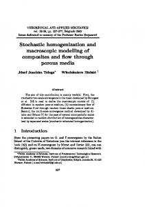
Next, we introduce the soccer example originally proposed in [23], and revisited in [4, 5, 7, 33, 47]. We illustrate both the transparency of the modelling mechanisms and ultimately the descriptive power this gives us in the context of problems which attempt to recreate some properties of a real system. The example is first formulated below as it appears in Littman’s paper [23], and then recreated in two different ways.

Fig. 2. The MDP adversarial soccer example from [23].

Formulation 3 (Littman’s adversarial MDP soccer). An early model of MDP style multiagent learning and referred to as soccer, the game is played on a 4  5 board of squares, with two agents (one of whom is holding the ball) and is zero-sum, see Fig. 6.2. Each agent is located at some grid reference, and chooses to move in one of the four cardinal points of the compass (N, S, E and W) or the P action at every time-step. Two agents cannot occupy the same square. The state space, SL1 , is of size 20  19  380, and the joint action space, AL1 B is a cartesian product of the two agents action spaces, AA L1  AL1 , and is of size 5  5  25. A game starts with agents in a random position in their own halves. The outcome for some joint action is generated by determining the outcome of each agent’s action separately, in a random order, and is deterministic otherwise. An agent moves when unobstructed and doesn’t when obstructed. If the agent with the ball tries to move into a square occupied by the other agent, then the ball changes hands. If the agent with the ball moves into the goal, then the game is restarted and the scoring agent gains a reward of 1 (the opposing agent getting
1). Therefore, other than the random turn ordering the game mechanics are deterministic. For example, see Fig. 3(a), here diagonally adjacent agents try to move into the same square: the order in which the agents act determines the outcome. The Littman soccer game can be recreated as a SMAFASP, with very little work. We add a couple more states for the reward function, add a trivial observation function, and flatten the turn-taking into the transition function. Formulation 4 (The SMAFASP soccer formulation). The SMAFASP formulation of the soccer game, is formed as follows: the state space SL2  SL1 sA sB , where sg is the state immediately after g scores a goal; the action space AL2  AL1 ; the observation space OL2  SL2 ; the observation function is the identity mapping; and the measure/reward function for agent A, f A P ΦpSL2 Ñ Rq is as follows, f A psA q  1,

f A psB q 
1,

and f A psq  0 for all other s P S.

21

(a)

(b)

Fig. 3. If agent A chooses to go East and agent B chooses to go South when diagonally adjacent as shown, the outcome will be non-deterministic depending on which agent’s move is calculated first. In the original Littman version this was achieved by resolving agent specific actions in a random order, fig. (a). In the SMAFASP version this is translated into a flat transition function with probabilities on arcs (square brackets), fig. (b). Agent B’s reward function is simply the inverse, i.e. f B psq 
f A psq, for all s. To define the transition function we need first to imagine that Littman’s set of transitions were written as agent specific transition functions, tg L1 P Σ pSL1AL1 Ñ SL1 q for each agent g — although this is not explicitly possible within the framework he uses, his description suggests he did indeed do this. The new transition function, tL2 P Σ pSL2AL2 Ñ SL2 q, would B B A then be defined, for all sn , sn 1 P SL1 , aA n P AL2 , an P AL2 , in the following way, tL2 psn

|sn , paAn, aBn qq

B A B ¸ tA L1 ps|sn , an q.tL1 psn 1 |s, an q  12 . . A B A tB L1 ps|sn , an q.tL1 psn 1 |s, an q sPS 1

L1

The transition probabilities involving the two new states, sA and sB , would be handled in the expected way. The turn-taking is absorbed so that the random order of actions within a turn is implicit within the probabilities of the transition function, see Fig. 3(b), rather than as before being a product of the implicit ordering of agent actions, as in Fig. 3(a). It is possible to reconstruct Littman’s game in a more flexible way. To see how, it is instructive to first examine what Littman’s motives may have been in constructing this problem, which may require some supposition on our part.Littman’s example is of particular interest to the multi-agent community, in that there is no independently optimal policy for either agent; instead each policy’s value is dependent on the opponent’s policy — therefore each agent is seeking a policy referred to as the best response to the other agent’s policy. Each agent is further limited by Littman’s random order mechanism, see Fig. 3(a), which means that while one agent is each turn choosing an action based on current state information, in effect the second agent to act is basing its action choice on state information that is one time-step off current; and because this ordering is random, neither agent can really rely on the current state information. Littman doesn’t have much control over this turn-taking, and as can be seen from the SMAFASP formulation, the properties of this turn-taking choice can be incorporated into the transition function probabilities (see Fig. 3 (b)). Different properties would lead to different probabilities in the SMAFASP, and would constitute a slightly different system with possibly different solutions. However, consider for example, that an agent is close to their own goal defending an attack. Its behaviour depends to some degree on where it expects to see its attacker next: the defender may wish to wait at one of these positions to ambush the other agent. The range of these positions is dependent on how many turns the attacker might take between these observations, which is in turn dependent on the turn-taking built into the system. For ease of

22

reading, we introduce an intermediate AMAFASP formulation. The individual agent action spaces are as in the SMAFASP, as is the observation space, but the new state information is enriched with the positional states of the previous time-step, which in turn can be used to generate the observations for agents. Formulation 5 (The first AMAFASP soccer formulation). This AMAFASP formulation of the soccer game, ML3 , is formed as follows: the new state space SL3  SL2  SL2 , so a new state at some time-step n, is given by the tuple psn , sn
1 q, where sn
1 , sn P SL2 and records the current and most recent positional states; there are two action space, one for A A A each agent, AA L3  AL2 and AL3  AL2 ; and two identical agent specific observation spaces, A B OL3  OL3  OL2 ; the new agent specific transition functions, tgL3 P Σ pSL3  AgL3 Ñ SL3 q, are defined, for all sn
1 , sn , s1n , sn 1 P SL2 , agn P AgL3 , in the following way: " g tL1 psn 1 |sn , agn q iff s1n  sn , tgL3 ppsn 1 , s1n q|psn , sn
1 q, agn q  0 otherwise. where tgL1 represents agent g’s deterministic action effects in Littman’s example, as in Formulation 4. The goal states, sA and sB , are dealt with as expected. g Recalling that OL3  SL2 , the observation function, ωL3 P Σ pSL3 Ñ OL3 q, is generated, for g all psn
1 , sn q P SL3 , on P OL3 , and g P tA, B u, in the following way, " iff sn
1  on , g ωL3 pon |psn , sn
1 qq  01 otherwise. The reward function is straightforward and left to the reader. Finally, we construct the turn-taking function uL3 P Σ pSL3 ÑtA, B uq, which simply generates either agent in an unbiased way at each time-step. The turn taking function is defined, for all psn , sn
1 q P SL3 , as uL3 pA|psn , sn
1 qq  uL3 pB |psn , sn
1 qq  1{ 2. This doesn’t fully replicate the Littman example, but satisfies the formulation in spirit in that agents are acting on potentially stale positional information, as well as dealing with an unpredictable opponent. In one sense, it better models hardware robots playing football, since all agents observe slightly out of date positional information, rather than a mix of some and not others. Both this and the Littman example do, however, share the distinction between turn ordering and game dynamics typified by Fig. 3 (a), what is more, this is now explicitly modelled by the turn-taking function. To fully recreate the mix of stale and fresh observations seen in Littman’s example along with the constrained turn-taking, we need for the state to include turn relevant information. This can be done with a tri-bit of information included with the other state information, to differentiate between; the start of a Littman time-step, when either agent could act next; when agent A has just acted in this time-step – and it must be B next; and vice versa when A must act next; we shall label these situations with l0 , lB and lA respectively. This has the knock on effect that in l0 labelled states the observation function is as Formulation 4; in lA and lB labelled states the stale observation is used – as in Formulation 5. Otherwise Formulation 6 is very much like formulation Formulation 5. Formulation 6 (The second AMAFASP soccer formulation). This AMAFASP formulation of the soccer game, ML4 , is formed as follows: there is a set of turn labels, L  tl0 , lA , lB u; the state space is a three way Cartesian product, SL4  SL2SL2L, where the parts can be thought of as current-positional-state, previous-positional-state and turn-label respectively; the action spaces and observation spaces are as before, i.e. AgL4  AgL3 , OL4  OL3 , for each agent g; the transition and reward functions are straightforward and are omitted for brevity; g the observation and turn taking functions are defined, for all psn , sn
1 , ln q P SL4 , on P OL4 and all agents g, in the following way,

# g ωL4

pon |psn , sn
1 , ln qq 

1 1 0

23

iff sn  on and ln  l0 , iff sn
1  on and ln  ug , otherwise.

and uL4 pgn |psn , sn
1 , ln qq 

#1 2

1 0

iff gn  g and ln  l0 , if gn  g and ln  ug , otherwise

The above formulation recreates Littman’s example precisely, and instead of the opaque turn-taking mechanism hidden in the textual description of the problem, it is transparently and explicitly modelled as part of the turn-taking function. So the Littman example can be recreated as a SMAFASP or AMAFASP, but more interestingly both AMAFASP formulations, 5 and 6, can be tuned or extended to yield new, equally valid, formulations. What is more, the intuitive construction means that these choices can be interpreted more easily. Consider Formulation 5; the turn-taking function u can be defined to give different turntaking probabilities at different states. For instance, if an agent is next to its own goal, we could increase its probability of acting (over the other agent being chosen) to reflect a defender behaving more fiercely when a loss is anticipated. Alternatively, if an agent’s position hasn’t changed since the last round, but the other’s has then the first agent could be more likely to act (possible as two steps of positional data are stored); giving an advantage to the P(ause) action, but otherwise encouraging a loose alternating agent mechanism. While Formulation 6 recreates the Littman example, it again can be adjusted to allow different choices to the turn taking mechanism; in particular it is now possible to enforce strictly alternating agents. This would be done by flipping from state label lA to lB or vice versa, at each step transition, and otherwise keeping things very much as before. It is important to note that many specific models built in this way, can be recreated by implicit encoding of probabilities within existing frameworks, but it is difficult to see how the experimenter would interpret the group of models as being members of a family of related systems. More importantly, agents can in general go any number of time-steps without being given the opportunity to act, whilst all the measure signals are generated at every time-step. Again, it would not be easy to recreate this without explicit state-based turn-taking.

6.3

Flexible Behaviour Regulation

If we increase the number of players in our game, we can consider increasing the number of measure functions for a finer degree of control over desired behaviour. With just 2 agents competing in the Littman problem, it is difficult to see how to interpret any extra signals, and adding agents will increase the state space and hence the policy size radically. So, before we address this aspect of the FASP formalisms, it is useful to examine a more recent derivative soccer game, namely Peshkin et al.’s partially observable identical payoff stochastic game (POIPSG) version [33], which is more amenable to scaling up.

Fig. 4. The POIPSG cooperative soccer example from [33].

Peshkin et al’s example is illustrated in Fig. 6.3. There are two team mates, V1 and V2 , and an opponent O, each agent has partial observability and can only see if the 4 horizontally and vertically adjacent squares are occupied, or not. Also, players V1 and V2 have an extra pass action when in possession of the ball. Otherwise the game is very much like Littman’s with joint actions being resolved for individual agents in some random order at each timestep. Contrary to expectations, the opponent is not modelled as a learning agent and doesn’t

24

receive a reward; instead the two team mates share a reward and learn to optimise team behaviour versus a static opponent policy; for more details see [33]. As with its progenitor, the Peshkin example could be simply reworked as a SMAFASP in much the same way as in Formulation 4. Recreating it as an AMAFASP is also reasonably straightforward; as before, the trick of including the previous step’s positional state in an AMAFASP state representation, allows us to generate stale observations – which are now also partial. As this is relatively similar to the Littman adaptions, the details are omitted. The focus here instead, is to show that, in the context of Peshkin’s example, a zero- or general-sum adaption with more agents, could have some utility. Firstly, agent O could receive the opposite reward as the shared reward of V1 and V2 , this could be done without introducing another measure function, merely reinterpreting Peshkin’s reward function; now, the opponent could learn to optimise against the cooperative team. More interestingly, the players V1 and V2 could be encouraged to learn different roles by rewarding V1 (say) more when the team scores a goal and penalising V2 more when the team concedes one, all this requires is a measure function for each agent and a zero-sum correction. It doesn’t stop there, we can add a second opponent (giving say O1 and O2 ), either rewarding them equally or encouraging different roles as with V1 and V2 . In this way we could explore the value of different reward structures by competing the teams. If more agents were added, even up to 11 players a side, and a much larger grid, the AMAFASP framework supports a much richer landscape of rewards and penalties, which can encourage individual roles within the team, while still differentiating between good and bad team collaborations. In this section, we have presented MDP style multi-agent examples from the literature, and shown how they can be reformulated as FASP type problems, including SMAFASP and AMAFASP. We have shown that state encapsulation is possible in practice, even with multi-agent examples, and that representations can be made more concise than the standard type1Ñtype2 POMDP transformation (see proof to Lemma 11. Of equal interest, we have shown that there are enriched formulations available to the FASP framework that are not naturally modelled by the other multi-agent MDP style frameworks encountered; further, these enriched formulations are relatively simple to construct and have intuitive interpretations.

7

Discussion

In this paper, we have shown that the different choices that have crept into the MDP and POMDP formalisms since first proposed, do not affect the fundamental nature or expressibility of the framework. To do this, we have tried to make explicit many assumptions about stochastically generated outcomes, which in turn may help implementers hoping to leverage the now vast body of MDP theory. As research has moved into multi-agent MDP style domains many of these assumptions and interpretations have come with it, and we hope that the work in the early sections of this paper has helped to clarify this. The paper then goes on to develop a more general, more intuitive set of tools for modelling MDP style problems, including (but not restricted to) multi-agent problems; and bases these tools on the tenet of transparent parsimonious mechanisms, an idea developed to encourage good modelling style. Transparent parsimonious mechanisms try to reflect common elements of real processes in understandable ways. We argue that state encapsulation facilitates adherence to such mechanisms, and informs all the ideas that follow. It allows frameworks that more naturally yield to analysis, and extension, but in such a way that it does not restrict existing models in any way — see Section 3. The purpose of this paper is not just to persuade modellers and experimenters to use state encapsulation, but also to encourage theorists to base analysis on state encapsulated systems. In some cases, this can simplify things conceptually and mathematically, and in turn may throw light on the properties of these problems. The preference for type2 POMDPs in the proofs in [19] is just one example of how state encapsulation leads to simpler analysis. In a future paper, we will demonstrate some of the analytical advantages of this approach. The first additional mechanism we add to the traditional POMDP is that of multiple measure functions. One measure signal for each measurable quantity fed to the agent or agents is then used to develop the FASP framework, and is more a challenge to theorists and experimenters alike to start examining a richer domain of problems; models that are easier to develop, and

25

better reflect the task at hand. The paper concentrates on multi-agent problems, and so defines a subtype of the FASP called the SMAFASP. Multi-agent problems have received a great deal of attention in the last few years, but lack emphasis on the general-sum stochastic game which allows more interesting agent relationships to be tested, including those that are mutually beneficial to multiple agents, so the paper explicitly develops a number of reward scenarios to encourage modellers to experiment with more interesting motivational relationships than straightforward cooperation or competition. We also argue, that treating communication actions separately from other (doing) actions — as proposed in a number of recent papers [30] [34] [35] and [48] — is difficult to reconcile with the principle of parsimony, since any action that changes the external environment can pass information to other agents, and any communication that has some physical component — radio, sound, light — changes the external environment: there is a false duality here, that may omit solutions which communicate with doing actions or vice versa. We would argue that the job of modelling other agents is best decoupled from the dynamics of the environment, and, if done explicitly, performed separately within each agents’ policy mechanism. This challenges us to develop better tools for agent communication: an idea we hope to visit in a later paper. At the same time, we acknowledge that there are complexity savings to such choices, sometimes dramatic ones [35], and there are no barriers to developing a framework incorporating these explicit commuinication mechanisms, with some of the other ideas from this paper, such as state encapsulation or turn-taking. This rationale of transparency then leads us to propose the AMAFASP, where agents are allowed to act out of turn with each other, which can tackle a set of problems which is potentially even broader than synchronous multi-agent games. We later show how we can use this to model Littman’s soccer problem, in an arguably more natural and certainly more transparent way, and how this model can then be altered to explore the game more fully. There are other mechanisms which satisfy our tenets of good practice other than those seen in this paper, some already developed, and we are sure there are others to add. As an example of the former, consider the simulation of a broken actuator — put forward in Bowling and Veloso’s paper on Nash-equilibria for restricted agents [6] — this is handled by separate stochastic mapping from intended action to restricted action, ideal for models intended to explore failing agents. Another candidate mechanism is the extraneous action events from [36], an explicit mechanism for modelling random changes in state not due to agents actions — again this is normally encoded in the transition function. So there is scope to grow the FASP family of frameworks, the aim being to enable experimenters to model systems more naturally. Shoham et al.’s 2006 survey on multi-agent learning [38] asserts that different members of the multi-agent learning (MAL) community are guided by different motivations, and highlight 5 ‘buckets’ or rough objectives they feel most MAL research falls into. The paper is not wholely uncontentious [43], but if we were to take their conclusions as a guide we could identify research objectives in all 5 disciplines that would benefit from our modelling techniques. The models produced by the FASP framework are intended to model flexibly especially within the multi-agent learning community, so it should come as no surprise that we recommend our tools widely, but we acknowledge that this work needs to be hardened and extended if they are to have broad appeal.

References 1. Jonathan Baxter, Peter L. Bartlett, and Lex Weaver. Experiments with infinite-horizon, policy-gradient estimation, November 2001. 2. Jonathan Baxter, Lex Weaver, and Peter L. Bartlett. Direct Gradient-Based Reinforcement Learning II: Gradient Ascent Algorithms and Experiments. Technical report, Australian National University, November 1999. 3. Daniel S. Bernstein, Shiomo Zilberstein, and Neil Immerman. The complexity of decentralized control of markov decision processes. In Proceedings of the 16th Annual Conference on Uncertainty in Artificial Intelligence (UAI-00), pages 32–37, San Francisco, CA, 2000. Morgan Kaufmann. 4. Reinaldo A. C. Bianchi, Carlos H. C. Ribeiro, and Anna H. Reali Costa. Heuristic selection of actions in multiagent reinforcement learning. In Manuela M. Veloso, editor, IJCAI, pages 690–695, 2007.

26

5. Michael Bowling, Rune Jensen, and Manuela Veloso. A formalization of equilibria for multiagent planning. In Proceedings of the AAAI-2002 Workshop on Multiagent Planning, August 2002. 6. Michael Bowling and Manuela Veloso. Existence of Multiagent Equilibria with Limited Agents. Journal of Artificial Intelligence Research 22, 2004. Submitted in October. 7. Michael H. Bowling, Rune M. Jensen, and Manuela M. Veloso. Multiagent planning in the presence of multiple goals. In Planning in Intelligent Systems: Aspects, Motivations and Methods. John Wiley and Sons, Inc., 2005. 8. Michael H. Bowling and Manuela M. Veloso. Simultaneous adversarial multi-robot learning. In Georg Gottlob and Toby Walsh, editors, IJCAI, pages 699–704. Morgan Kaufmann, 2003. 9. Darius Braziunas. POMDP solution methods: a survey. Technical report, Department of Computer Science, University of Toronto, 2003. 10. Anthony R. Cassandra. Optimal policies for partially observable markov decision processes. Technical report, Brown University, Providence, RI, USA, 1994. 11. Anthony R. Cassandra, Leslie Pack Kaelbling, and Michael L. Littman. Acting optimally in partially observable stochastic domains. In Proceedings of the Twelfth National Conference on Artificial Intelligence (AAAI-94), volume 2, pages 1023–1028, Seattle, Washington, USA, 1994. AAAI Press/MIT Press. 12. Tony Cassandra. The POMDP Page. URL, 2003-2005. 13. Shih-Fen Cheng, Evan Leung, Kevin M. Lochner, Kevin O’Malley, Daniel M. Reeves, Julian L. Schvartzman, and Michael P. Wellman. Walverine: a walrasian trading agent. Decis. Support Syst., 39(2):169–184, 2005. 14. Alain Dutech, Olivier Buffet, and Francois Charpillet. Multi-agent systems by incremental gradient reinforcement learning. In IJCAI, pages 833–838, 2001. 15. Jerzy Filar and Koos Vrieze. Competitive Markov decision processes. Springer-Verlag New York, Inc., New York, NY, USA, 1996. 16. P. Gmytrasiewicz and P. Doshi. A framework for sequential planning in multi-agent settings, 2004. 17. Amy Greenwald and Keith Hall. Correlated q-learning. In AAAI Spring Symposium Workshop on Collaborative Learning Agents, 2002. 18. Junling Hu and Michael P. Wellman. Multiagent reinforcement learning: theoretical framework and an algorithm. In Proc. 15th International Conf. on Machine Learning, pages 242–250. Morgan Kaufmann, San Francisco, CA, 1998. 19. Tommi Jaakkola, Satinder P. Singh, and Michael I. Jordan. Reinforcement learning algorithm for partially observable Markov decision problems. In G. Tesauro, D. Touretzky, and T. Leen, editors, Advances in Neural Information Processing Systems, volume 7, pages 345–352. The MIT Press, 1995. 20. Leslie Pack Kaelbling, Michael L. Littman, and Anthony R. Cassandra. Planning and acting in partially observable stochastic domains. Technical Report CS-96-08, Brown University, 1996. 21. Vijay R. Konda and John N. Tsitsiklis. On actor-critic algorithms. SIAM J. Control Optim., 42(4):1143–1166, 2003. 22. Martin Lauer and Martin Riedmiller. An algorithm for distributed reinforcement learning in cooperative multi-agent systems. In Proc. 17th International Conf. on Machine Learning, pages 535–542. Morgan Kaufmann, San Francisco, CA, 2000. 23. Michael L. Littman. Markov games as a framework for multi-agent reinforcement learning. In Proceedings of the 11th International Conference on Machine Learning (ML-94), pages 157–163, New Brunswick, NJ, 1994. Morgan Kaufmann. 24. Michael L. Littman. The witness algorithm: Solving partially observable markov decision processes. Technical Report CS-94-40, Brown University Department of Computing, 1994. 25. John Loch and Satinder P. Singh. Using Eligibility Traces to Find the Best Memoryless Policy in Partially Observable Markov Decision Processes. In Proc. 15th International Conf. on Machine Learning, pages 323–331. Morgan Kaufmann, San Francisco, CA, 1998. 26. Sridhar Mahadevan. Average reward reinforcement learning: Foundations, algorithms, and empirical results. Machine Learning, 22(1-3):159–195, 1996.

27

27. Stephen McGough, Asif Akram, Li Guo, Marko Krznaric, Luke Dickens, David Colling, Janusz Martyniak, Roger Powell, and Paul Kyberd. GRIDCC: Real-time Workflow System. In The 2nd Workshop on Workflows in Support of Large-Scale Science, June 2007. 28. Tom M. Mitchell. Machine Learning. McGraw-Hill, New York, 1997. 29. George E. Monahan. A survey of partially observable markov decision processes: Theory, models, and algorithms. Management Science, 28(1):1–16, Jan 1982. 30. Ranjit Nair, Milind Tambe, Makoto Yokoo, David V. Pynadath, and Stacy Marsella. Taming decentralized pomdps: Towards efficient policy computation for multiagent settings. In Georg Gottlob and Toby Walsh, editors, IJCAI, pages 705–711. Morgan Kaufmann, 2003. 31. Fans Oliehoek and Arnoud Visser. A Hierarchical Model for Decentralized Fighting of Large Scale Urban Fires. In P. Stone and G. Weiss, editors, Proceedings of the Fifth International Conference on Autonomous Agents and Multiagent Systems (AAMAS), Hakodate, Japan, May 2006. 32. A. Papoulis. Probability, Random Variables, and Stochastic Processes. McGraw Hill, 3rd edition, 1991. 33. Leonid Peshkin, Kee-Eung Kim, Nicolas Meuleau, and Leslie P. Kaelbling. Learning to cooperate via policy search. In Sixteenth Conference on Uncertainty in Artificial Intelligence, pages 307–314, San Francisco, CA, 2000. Morgan Kaufmann. 34. D. Pynadath and M. Tambe. The communicative multiagent team decision problem: analyzing teamwork theories and models, 2002. 35. D. Pynadath and M. Tambe. Multiagent teamwork: Analyzing the optimality and complexity of key theories and models, 2002. 36. Bharaneedharan Rathnasabapathy and Piotr Gmytrasiewicz. Formalizing multi-agent pomdp’s in the context of network routing. 37. Maayan Roth, Reid Simmons, and Manuela Veloso. What to communicate? executiontime decision in Multi-agent POMDPs. 38. Yoav Shoham, Rob Powers, and Trond Grenager. If multi-agent learning is the answer, what is the question? Artif. Intell., 171(7):365–377, 2007. 39. Satinder P. Singh, Tommi Jaakkola, and Michael I. Jordan. Learning without stateestimation in partially observable markovian decision processes. In International Conference on Machine Learning, pages 284–292, 1994. 40. Satinder P. Singh and Richard S. Sutton. Reinforcement learning with replacing eligibility traces. Machine Learning, 22(1–3):123–158, 1996. 41. Richard D. Smallwood and Edward J. Sondik. The Optimal Control of Partially Observable Markov Processes over a Finite Horizon. Operations Research, 21(5):1071–1088, Sep-Oct 1973. 42. Matthijs T.J. Spaan and Nikos Vlassis. A point-based POMDP algorithm for robot planning. In Proceedings of the IEEE International Conference on Robotics and Automation, pages 2399–2404, New Orleans, Louisiana, April 2004. 43. Peter Stone. Multiagent learning is not the answer. It is the question. Artificial Intelligence, 2006. To appear. 44. R. Sutton, D. McAllester, S. Singh, and Y. Mansour. Policy gradient methods for reinforcement learning with function approximation, 1999. 45. R.S. Sutton and A.G. Barto. Reinforcement Learning: An Introduction. MIT Press, Cambridge, MA, 1998. 46. Gerald Tesauro. Temporal difference learning and td-gammon. Commun. ACM, 38(3):58–68, 1995. 47. William T. B. Uther and Manuela M. Veloso. Adversarial reinforcement learning. Technical report, Computer Science Department, Carnegie Mellon University, April 1997. 48. P. Xuan, V. Lesser, and S. Zilberstein. Communication in multi-agent markov decision processes, 2000. 49. Erfu Yang and Dongbing Gu. Multiagent reinforcement learning for multi-robot systems: A survey. Technical report, University of Essex, 2003. 50. Martin Zinkevich, Amy Greenwald, and Michael Littman. Cyclic equilibria in markov games. In Y. Weiss, B. Sch¨ olkopf, and J. Platt, editors, Advances in Neural Information Processing Systems 18, pages 1641–1648. MIT Press, Cambridge, MA, 2005.

28

A

Additional proof for inverse bijective function

Lemma 17 (The Policy Mapping b, as defined in proof to thm. 1, is bijective). If we have an AMAFASP M and FASP M 1 as defined in the proof to thm. 1 then there is an inverse b
1 : Π 1 Ñ Π, and for all g P G, ogi P Og , agj P Ag , π P Π and ok P O1 , such that ok  p. . . , ogi , . . .q, i.e. ogi  ogk , then 





b pπ q  π 1


1 1 g g P Π1 Ñ  b pπ qpaj |oi q 

¸

π g pagj |ogi q 

 π 1 pal |ok q

P 1

al A

al

p...,agj ,...q

. Proof. For ease of reading we will define the following notation, for all g ag P Ag , o P O1 , a P A1 , and π P Π, such that; bpπ q  π 1 P Π 1 , further then,

P G, og P Og ,

π g pag |og q  πogg

ag

and

1

π 1 pa|oq  π o1 o2 ...o|G|

| |

a1 a2 ...a G

It is therefore clear from our definition of b, that ¹ 1 |G| πogg  πo11 .π o22 . . . π o|G| π o1 o2 ...o|G| 

| |

P

a1 a2 ...a G

g G

a1

ag

| |

a2

aG

P Ai , knowing that

And if we were to sum this over all agent i specific actions, ai 1, then,

¸ ai

P

Ai

1

π o1 o2 ...o|G|

| |

a1 a2 ...a G



¸ ai

P

Ai

 πa1

o1 1

a2

i 1

2

| |

ai




ai 1



aG

¸

P





P

P

i j ai Ai

a A

 

¸ ¸

i

ai Ai

|G|

.π oi i 11 . . . π o|G|

πoi

ai

| |

ai 1

aG

|G|

1 .π oi i 11 . . . π o|G| .π o22 . . . π oi
i
1 a2




ai 1

ai 1

Clearly, performing this sum for all agents except agent j ¸ ¸ ¸ 1 π o1 o2 ...o|G| π 1 pa|oq  fixing aj



|G|

a1

 πao1 .πao2 . . . πo
i
1 . 1

i P πaoii

ai Ai

πo11 .π o22 . . . π oi i . . . π o|G|

2

1

°

| |

aG

P G, we get,

| |

a1 a2 ...a G

|G|

πo11 . . . π o|G| a i j ai PAi 1  a|G|  ¸ ¸ 1 2 πo1 . πo2 . . . a1 a2 a1 PA1 a2 PA2    ¸ j
1 j ... πoj
1 .π oj .


P


aj 1 Aj 1




aj 1

aj

¸

P

 j 1

πoj

...

π a  πj poj , aj q

...

¸

| | PA|G|

aG

j

1

aj 1 1 aj 1 Aj 

|G| π



| | | |

o G

aG

oj j

and we are back at the single values for individual agents, as required, and hence b is bijective. [\

29