MEMS IMU Stochastic Error Modelling

MEMS IMU Stochastic Error Modelling Elder M. Hemerly* [email protected] *Technological Institute of Aeronautics, Systems and Control Department, São José dos Campos – São Paulo, Brazil Abstract: Low cost inertial measurement units (IMU) are comprised of micro-electro-mechanical systems (MEMS) gyroscopes and accelerometers. These inertial sensors have high random noise and time varying bias. Hence, an accurate stochastic error model is necessary to predict performance and also to implement an attitude and heading reference system (AHRS) or a navigator. The parameters of this stochastic model are classically obtained via Allan Variance analysis. In this paper two modern approaches, based on autoregressive moving average (ARMA) model and Kalman Filter, respectively, are investigated and their performances are unveiled via sensitivity analysis, realistic simulations with typical MEMS parameters and also with experimental data. Basic equations for the estimation problem are developed and the solution sensitivity to data and parameters is discussed. It is shown that the deficiency with the online methods can be traced back to the difficulty in estimating the parameters B (bias instability) and K (rate random walk for gyros, acceleration random walk for accelerometers) separately under high measurement noise N (angular random walk for gyros, velocity random walk for accelerometers), which is typical of MEMS IMU. Keywords: System modelling, state estimation, time series analysis, data modelling and estimation.

1- Introduction Due to its low cost, MEMS IMU has been extensively used in the implementation of inertial navigation systems (INS). See, for instance, [1-3]. The accuracy of these systems depends on the adequate error modeling of the IMU sensors. This error model is actually divided into two parts: a) a deterministic or systematic model, and b) a stochastic model. The deterministic model encapsulates the biases, scale factors and misalignments errors. The parameters associated to the deterministic error model can be obtained by two different approaches: 1) static procedure in a laboratory environment, such as in [4] and 2) identification based procedure, with a cost function which incorporates the unknown parameters. See [5] for details. In both cases, if the gyroscope does not measure the Earth’s angular velocity, as is usually the case with MEMS sensors, then a rotating table is required for calibration. Once the deterministic IMU model is obtained, the remaining error has stochastic

nature and must be modeled accordingly. For a detailed definition of all the parameters in this stochastic model, see IEEE Std. 952-1997 [6], which also recommends the Allan Variance method for experimentally obtaining these parameters. This model can then be used, for instance, to implement INS based navigators, such as in [7] and [8]. A comprehensive example of the classical approach for stochastic error modeling, based on Allan Variance analysis, is [9]. Experimental works conducted there indicated that MEMS gyroscope stochastic error model is mainly composed of: a) bias instability (B), which represents a time varying bias modeled by a first order GaussMarkov process; b) angular random walk (N), which is an angular error due to white noise in the angular rate, and c) rate random walk (K), representing a rate error due to white noise in angular acceleration. These parameters are also the most relevant for accelerometers, except for the change in physical meanings: N is velocity random walk, and K is the acceleration random

walk. In [10], the statistical properties of the estimates obtained via Allan Variance analysis is carefully investigated, by considering tactical-grade MEMS gyros. These sensors are easier to tackle than those considered by [9], since an accurate model can be obtained with only 2 parameters: N (angular random walk) and K (rate random walk). Despite its broad application to IMU stochastic error modeling, the classical approach, based on Allan Variance analysis, is not an automatic procedure. It does require some interaction with the user, for determining adequate asymptotes to the Allan graphics: accordingly to the IEEE standard [6], each parameter in the error model has a distinctive signature in the Allan graphics. For instance, the parameters N and K are associated with asymptotes having slopes -1/2 and 1/2, respectively. Some procedures have then been proposed to estimate automatically the parameters associated to the IMU stochastic error model. In [11], it is shown that a combination of several different noises can be described by a single ARMA model, by properly calculating the parameters of the equivalent correlated noise. It is argued that for ring laser gyroscope (RLG), by considering only N (angular random walk) and Q (quantization noise), the performance is similar to the Allan approach and the implementation is simpler. In [12], the equivalent ARMA model representation proposed by [11] is employed as departing point, but the input/output model is rewritten in the state space form. MEMS sensors are considered, instead of RLG, hence there are 4 parameters associated to the stochastic error model: bias instability (B), angular random walk (N), rate random walk (K) and rate ramp noise (R). The problem then boils down to a state estimation problem, where the dynamic matrix A, the output matrix C and the measurement intensity noise are unknown.

The solution is implemented via the EM (Expectation Maximization) algorithm, which solves the ensuing MLE (Maximum Likelihood Estimation) problem. It is concluded that the proposed online method avoids the storage of data and produce results within the error limits of Allan Variance analysis. It should be noted that the number of parameters to be retained in the IMU stochastic model depends on the fabrication technology: [9] considers 3 parameters, [10]-[11] only 2 and [12] employs 4 parameters. In general, the better the technology, the lesser the number of parameters required in the model. In this work, MEMS gyros similar to those investigated in [9] are considered, i.e., the most relevant parameters in the stochastic model are B, N and K. The goal is to investigate if the modern approaches for IMU stochastic modeling, such as those proposed by [11] and [12], do provide reliable alternative to the classical approach base on Allan Variance analysis, such as in [9]. As a first step, the approaches in [11] and [12] are tailored to the 3 parameters model employed by [9]. The main contributions are: 1) detailed sensitivity analysis of the estimates to the data and underlying parameters, which was not carried out in [11] and [12]; 2) comparative performance evaluation of classical and modern approaches, by using realistic simulations with typical MEMS gyros parameters, and experimental data. This has not been done by [9]-[12], and 3) light is shed on the online methods deficiency in the present case, by tracing it back to the difficulty in estimating the parameters B and K separately under the typical high measurement noise N exhibited by MEMS IMU.

2- Equivalent ARMA Model Approach In this paper this method is applied to the MEMS IMU modeling, with the 3 main paramters B, N and K, already discussed in section 1. However, at first the simpler case of [11] is considered, where only the parameters N (angle random walk) and Q (quantization noise) is revisited, for correcting a typo error and preliminary performance evaluation. In order to obtain the equivalent ARMA model in this simpler case, recall that in the discrete time domain the contributions of the error sources in the gyro measurement are, respectively, y arw (k)  1w1 (k) , w1 (k) ~ N(0,1) (2.1)

y q (k )   2 ( w 2 (k )  w 2 (k - 1)) , w 2 (k ) ~ N(0,1)

(2.2)

where the standard deviations 1 and  2 depend on the parameters N and B as indicated in [12]. Then, by defining the measurement as

y(k )  y arw (k )  y q (k )  1w1 (k )   2 (w 2 (k) - w 2 (k - 1))

(2.3)

the application of the equivalent ARMA model representation to the right hand side of (2.3), which comprises two different noises, produces the equivalent model, with just one noise, y(k)  e0 w(k)  e1w(k - 1) , w(k) ~ N(0,1) (2.4)

which is an ARMA model with structure (0,1). In (2.4), the values of the parameters e 0 and e1 are obtained by imposing equal correlation coefficients to the right hand sides in (2.3) and (2.4). This produces the relations

root inside the unit circle. The solution of (2.5) presented in equation (9) of [11] is incorrect. The correct solution is e0 

(12  222 )  1 12  422

e1  

2 2 22

(12



222 )  1

12



,

422

(2.6)

The simulation from [11] is now reproduced with the corrected relations (2.6). In this case, the standard deviations associated to the angle random walk and the quantization noise are, respectively, 1  35.6 deg/s and 2  114.525 deg/s , and the sampling time is T=0.01s. With these values, the true parameters in the equivalent ARMA model (2.4) are, accordingly to (2.6), e0  133.7 and e1  -98.1 . Table 1 displays the errors in percent, as functions of the number of readings, obtained from a Monte Carlo simulation. In these simulations, the ARMA model identification was carried out by using the armax() command from Matlab, since the identification problem is not the main issue in this paper. Table 1: Equivalent ARMA modeling performance for the simple ARMA (0,1) model. Number of readings

Percent error in

Percent error in

e 0 estimation

e1 estimation

100

4.907

11.558

1000

2.476

4.147

10000

0.543

1.455

12  222  e02  e12 and  22  e0e1 (2.5) with the constraint that the polynomial C(q 1 )  e0  e1q 1 , where q 1 is the backward shift operator, is stable, i.e., has

From Table 1 it can be concluded that the equivalent ARMA modeling is quite efficient for the 2 parameters (N and Q)

model: good performance is obtained even with a small number of measurements. The problem now is to see if this good performance is also exhibited for the MEMS IMU stochastic modeling, where there are 3 parameters (B, N and K), instead of 2 (N and Q, which is the case shown in Table 1). The problem here does not lie only on the number of parameters, but mainly on their physical meaning. See IEEE Std. 952-1997 [6] for details.

With this proviso, from (2.7)-(2.10) and (2.12) the measurement equation is rewritten as the stationary process y d (k )  y d (k  1)  1 ( w1 (k  1)  w1 (k  2))   2 w 2 (k )   2 (1  ) w 2 (k  1)   2 w 2 (k  2)   3 w 3 (k  1)  3 w 3 (k  2)

(2.13) Hence the equivalent ARMA model has order (1,2), i.e., y d (k )  y d (k  1)  e 0 w (k )  e1w (k  1) 

2.1- Equivalent ARMA Model for MEMS IMU Instead of (2.3), now the MEMS IMU model must comprise, as in [9], the contributions of bias instability, angle random walk and rate random walk, i.e., the gyro measurement is given by y(k)  ybi (k)  yarw (k)  yrrw (k)

y bi (k )  y bi (k  1)  1w1 (k  1) , w1 (k ) ~ N(0,1)

(2.7) (2.8)

y arw (k)   2 w 2 (k) , w 2 (k) ~ (0,1) (2.9)

y rrw (k )  y rrw (k  1)   3 w 3 (k  1) , w 3 (k ) ~ N(0,1) (2.10) In (2.8) the parameter  is obtained by discretizing the continuous time first order Gauss-Markov process, i.e.,   e T ,   1/ ,

 : correlation time (2.11)

and the standard deviations 1 ,  2 and  3 are related to the parameters B, N and K as in [12]. Since the rate random walk (2.10) is a non-stationary process, instead of taking (2.7) as being the gyro measurement, it is advisable to consider as measurement the difference yd (k)  y(k)  y(k  1)

(2.12)

e 2 w (k  2) , w(k) ~ N(0,1)

(2.14) and by calculating the correlations, the relations between the standard deviations and the MA parameters in (2.14) are



 

212  2  2  2 2  22  (1   2 ) 32  e 02  e12  e 22



 12  1  2   2  22  e 0 e 2

2 2

 32  e 0 e1  e1e 2

(2.15)

The MEMS IMU stochastic error modeling then boils down to the following problem: given the gyro measurements (2.12), estimate the parameters ( e0 , e 1 , e 2 ) in the ARMA model (2.14) and then get the standard deviations ( 1 , 2 , 3 ) from (2.15). The constraints here are: a) the parameter  must be positive, from (2.11), and b) the polynomial C(q 1 )  e0  e1q 1  e2q 2 must be stable, i.e., must have roots inside the unit circle. The estimation of the parameter  in (2.15) comes directly from the identified ARMA model, due to (2.14). Hence, (2.15) corresponds to an algebraic system with 3 equations and 3 unknowns ( 1 , 2 , 3 ), from which the parameters B, N and K of the stochastic error model are finally obtained.

Just to recall, given gyro measurements (2.12), the ARMA model (2.14) is identified, thereby providing estimates for  , e0 , e 1 and e 2 . With these values, from (2.15) the standard deviations 1 , 2 and 3 are obtained, and then parameters which define the stochastic error model, namely B, N and K. However, for performance analysis, it is better to proceed the other way round: generate simulated data with given values for B, N, K and  , then obtain e0 , e 1 and e 2 from (2.15). These are the true parameters associated to the equivalent ARMA model. Hence, good performance is obtained if the ARMA identification algorithm provides estimates close enough to the true values of e0 , e 1 and e 2 . A typical MEMS gyro is considered, with parameters given by [9] as B  1.55x102 deg/s , N  5.75x102 deg/s 1/2 and K  9x104 deg/s 3/2 . By assuming correlation time equal to 100 s and sampling time equal to 0.01s, the true values for e0 , e 1 and e 2 can be obtained from (2.15) in the following way: remove e0 and e 1 from the last 2 equations in (2.15) and substitute them into the first equation in (2.15). An algebraic equation of order 8 for e 2 is obtained, with even powers only. Hence, this equation can be reduced to order 4. A total of 8 roots are produced, but only the positive solutions are of interest, and each one must be tested for the constraint that C(q1)  e0  e1q1  e2q2 is Hurwitz. Let e0 , e1 and e 2 be the viable solution. Now, suppose that, as an ideal case, the identification algorithm produces exactly the true viable solution e0 , e 1 and e 2 . Then, 2 is easily calculated by using the last equation in (2.15), and from the first 2 equations, 1 and  3 are given by

2    e e  e   1   2 22  , M  12    2 12 0 2 2 2 2 3  e0  e1  e2  2 1     2    1 (2.16) M 2  2 1   









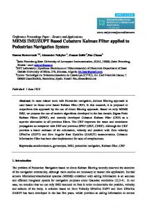
From (2.16), the solutions for 1 and  3 depend critically on the matrix M condition number. In this particular example,   1/100  0.01s and T=0.01s. From (2.11),   0.9999 , which implies cond(M)  109 . Hence, the system of equations (2.16) is very badly conditioned and the parameters 1 and  3 cannot be determined separately with accuracy. This conclusion is completely independent of the identification algorithm accuracy, hence the number of gyro measurements. More precisely, increasing the number of readings will not change the scenario. Figure 1 shows the matrix M condition number as function of the gyro correlation time and the sampling time, both in seconds. Condition number as function of correlation time and sampling time 9 8 T=0.01s 7 6

log(cond)

2.2- Simulation Results

T=0.1s 5 4 T=1s 3 2 1

0

10

20

30 40 50 60 70 Correlation time, in seconds

80

90

Figure 1: Condition number of M in (2.16), in log10 , as function of the correlation time   1/  and sampling time T. From Figure 1 it is concluded that matrix M is only well conditioned if the correlation time is small and the sampling

100

time is large. This mathematical difficulty in obtaining 1 and  3 separately with accuracy can be physically explained by 2 different factors: a) the rate random walk variance increases as the sampling time decreases, and b) for small values of  and T, from (2.11) it follows that  is close to 1, hence the first order Gauss-Markov process (2.8) does not differ too much from the random walk process (2.10). More precisely, the problem boils down to estimating two quite close parameters under high noise condition. Indeed, recall that for MEMS IMU the parameter N (angle random walk) is large, hence 2 is large in (2.9). Consequently, the measurement (2.12) is very noisy. With the previously defined values of B, N, K,  and T, 100000 readings were generated by using (2.7)-(2.12), which would correspond to an acquisition time of 16.167 minutes. By using the Matlab armax() command for identification, the only parameter which was correctly estimated was  2 , from which the estimate ˆ  0.0574 was obtained. This represents an N error of only 0.212 % with respect to the true value of N. The estimate of  was ˆ =0.9783, which is close to 1, as expected, but the signal is incorrect. The values for B and K were incorrect by orders of magnitude. Hence, a comparison with the Allan Variance analysis is necessary. The corresponding Allan graphic, for the same realization, is shown in Figure 2.

Figure 2: Allan graphic and asymptote lines with inclinations +1/2, 0 and -1/2, for estimating N, B and K, respectively. From Figure 2, the estimates obtained from Allan Variance analysis are ˆ  5.6x102 , ˆ  1.2x102 and N B 3 ˆ K  1.1x10 . Hence, the error in percent are, respectively, 2.6%, 22.5% and 18.2% . Therefore, the results from the Allan Variance analysis are good for N and reasonable for B and K, whereas the results from the equivalent ARMA modeling are very good for N and useless for B and K. It is then concluded that Allan Variance is a better approach in the present case. Remark 1: A potential cause for the error in the estimation of  in the equivalent ARMA approach could be the presence of correlated noise in (2.14). Hence, trails were carried out by employing the instrumental variable identification algorithm, by means of the ivar() command from Matlab. However, the results were equally incorrect, perhaps due to the high noise content of the measurement signal (2.12), which is, as already pointed out, the usual case when MEMS gyros are employed. Remark 2: An additional attempt was made to improve the estimate of  by using a constrained identification scheme, since it is known from the outset that this parameter is

Remark 3: The sampling time was then increased to T=1s, which implies an acquisition time of 27.77 hours. The performance did not improve for the equivalent ARMA model. Several other simulations, varying the number of data points, sampling time and so on did not alter the conclusion: the equivalent ARMA model is not applicable for estimating simultaneously the parameters N, B and K associated to the stochastic error model of a MEMS gyro. 2.3- Simplified Model Due to the inadequate performance reported in section 2.2, a particular case is now considered, by dropping the parameter K from the MEMS gyro stochastic error model. This case is still relevant and simplifies the problem considerably, since the nonstationarity caused by (2.10) is removed. With this simplification, the equivalent MA part of the ARMA model is as in section 2, i.e., C(q 1 )  e 0  e1q 1 , but instead of (2.5), the algebraic system of equations is now 12  (1   2 ) 22  e 02  e12 ,

  22  e 0 e1

associated to the parameter  estimation, as function of the sampling time, is shown in Figure 3. Correlation time estimation error as function of the sampling time 50 45 40

Error in percent

positive, according to (2.11). Again, this procedure was not reliable, due to the high measurement noise.

35 30 25 20 15 10 0.02

0.03

0.04

0.05 0.06 0.07 Sampling time in seconds

0.08

0.09

0.1

Figure 3: Parameter  estimation error, in percent, as function of the sampling time. For T=0.1s, several realizations were considered and a typical estimation result ˆ  5.74x102 , B ˆ  1.52x102 and was N ˆ =0.9992, with in percent errors 0.21%, 2.17% and 0.02%, respectively. Hence, by considering simplified MEMS gyros model with only parameters B and N, it is concluded that the equivalent ARMA modeling is efficient for estimating these parameters, if large enough sampling time is employed.

(2.17) whose solution is much simpler than the system (2.15). By generating 100000 readings with the true parameters values B, N,  and T, the MATLAB armax() command produced inadequate result for the estimate of  . The problem now is not caused by almost singularity in the algebraic equation system (2.17), but solely by the high measurement noise. The sampling time was then increased from 0.02s to 0.1s, for reducing the random walk variance. The error in percent

3- Kalman Filter Approach Another modern approach for IMU stochastic modeling is proposed by Saini [12]. The departing point is the equivalent ARMA approach proposed by [11], but [12] formulates the problem in the continuous time domain and employs state space representation. By considering the model with parameters B, N, K and  as in section 2, the equivalent ARMA model is given by y(t )  y (t )  K 2   2 B 2 w  (t )  Kw(t )

(3.1)

which can be rewritten in state space form and discretized via Euler method, with small enough sampling time T, as in [12], according to T  1 x (k  1)    x (k )  w (k ) 0 1  T



y(k )  K



K 2   2 B 2 x (k ) 

(3.2) N T

v( k )

(3.3) where, for small enough T, the state noise covariance matrix is given by T

Pw   e At Bw( t )dt  BB T T , 0

with

B  [0 1]T .

Remark 1: Model (3.2)-(3.3) differs from (2.14) in the sense that the rate random walk pole at z=1 has not been removed by data differencing. This explains why (3.2) is a second order model, whereas (2.14) is a first order system. Remark 2: Technically, the problem of estimating B, N, K and  given (3.2)-(3.3) constitutes an adaptive state estimation problem, i.e., joint estimation of state and parameters. The main difficulty here arises from the following fact: in (3.3), the intensity of the measurement noise v(k) depends on the unknown parameter N. Hence, the measurement noise covariance matrix is not known. Therefore, the usual approach for implementing adaptive state estimation, namely the one base on state augmentation and extended Kalman Filter, can not be applied directly. Remark 3: In [12], the adaptive state estimation problem posed by (3.2)-(3.3) is solved by using the EM (Expectation Maximization), see [12] for details. Several sensitivities must be calculated, i.e., the ensuing algorithm is much more complicated than the Kalman Filter. Remark 4: From all the cases considered in section 2, i.e., for MEMS IMU, the estimation of the angle random walk N can

be easily accomplished, since it is the parameter which influences the output the most. As a matter of fact, a simple sample variance can provide accurate results. For instance, by using the same parameters B, N, K,  and T in section 2.2, with 500, 1000 and 6000 data points the error in percent associated to the estimation of N was 3.47%, 3.02% and 0.63%, respectively. Hence, in 1 minute (6000*0.01=60s) it is possible to obtain a good enough estimate for N. Indeed, the data acquired to estimate N has to correspond to a short amount of time, otherwise B and K can display their effects, thereby spoiling the estimate of N. Based on Remarks 2-4, the following simplified and much simpler version of [12] is investigated for estimating the parameters B, N, K and  associated to the MEMS gyro stochastic error model: Step 1: By using initial data, estimate N by calculating the sample mean variance. Step 2: Given the previous estimate of N, the adaptive estimation problem posed by (3.2)-(3.3) can be solved by the Extended Kalman Filter with augmented state x a  [x T B K ]T  R 5 , x  R 2

(3.4)

where x(k) is defined in (3.2). For implementing the EKF, it is also supposed that the unknown parameters B, K and  are modeled as constants. With the previous assumptions, the linearized system to which the Kalman Filter is applied has dynamic and output matrices defined by    A   

1

T

0

0

0 0

1  Tx 5 (k ) 0

0 1

0 0

0 0

0 0

0 0

1 0

0   Tx 2 (k )   0  0   1

, C  c1 c2 c3 c4 c5 

r  x 24 (k)  x 32 (k)x 52 (k) , c1  x 4 (k)x 5 (k) ,

c 2  r , c 3  (1 / r)x 2 (k)x 3 (k)x 52 (k)

c 4  x1 (k)x 5 (k)  (1 / r)x 2 (k)x 4 (k) ,

c 5  x 1 (k ) x 4 (k )

 (1 / r)x 2 (k)x 32 (k)x 5 (k)

(3.5) Simulations where carried out by generating data with the same parameters B, N, K,  and T as in section 2, and the performance was highly dependent on the realization. The explanation was found in the very badly conditioning of the observability matrix of the linearized model. Indeed, its condition number was of order 1022 . Similar difficulty has already been encountered in section 2.2, where it was concluded that the separate estimation of the parameters B and K is not reliable. In [12] this observability issue is not even addressed.

4- Experimental Results Experimental data from a MEMS gyro was obtained, by using the mAHRS, from Innalabs. Only raw roll gyro data is considered, with 130000 samples, acquired at 100Hz. The Allan graphic is shown in Figure 4.

Figure 4: Allan graphic and asymptote lines with inclinations +1/2, 0 and -1/2, for estimating N, B and K, respectively, by using experimental data from mAHRSInnalabs roll gyro.

From Figure 4, the estimates for N, B and K obtained from Allan Variance analysis, by using the asymptote lines, are ˆ  2.95x102 deg/s 1/2 , B ˆ  1.74x10 2 deg/s , N ˆ  5.2x103 deg/s 3/2 . The estimate for and K N looks adequate, since the sample variance, calculated with the first 1000 data points, produces the rough estimate 2.41x102 . These parameters have approximately the same magnitudes as those exhibited by the sensor employed in Petkov and Slavov (2010), hence are of the same MEMS class. By using now the equivalent ARMA model as in section 2.2, the estimated parameters turned out to be completely unreliable, for instance 1 1/2 ˆ . At least for the N  1.87x10 deg/s estimate of N, this result can be easily explained as follows: 1) the Matlab armax() command produces a final prediction error (FPE) equal to 0.0625. Hence, if all the noise effects were to come only from N, the estimated value would be 2 1/2 ˆ N  2.5x10 deg/s , which is coherent with ˆ  2.95x102 deg/s 1/2 estimated the value N via Allan Variance analysis; 2) in the equivalent ARMA modeling, the N estimate depends on 2 , which from (2.15) depends on the estimates of  , e0 and e 2 . But these 3 parameters are incorrectly estimated, despite several attempts of providing different initial estimates for the ARMA polynomials, via the the Matlab command idpol(). For the Kalman Filter approach, the estimate for N was obtained as in Remark 4, ˆ  2.41x102 deg/s 1/2 . Several tests i.e., N were performed by varying the initial estimates for B and K. The values obtained via Allan Variance analysis were used as references. The conclusions were the following: a) the estimates for B do not vary much around their initial estimates, and b) the estimates for K are more sensitive to the data, but converge to values which are

dependent on the initial estimates. This suggests the experimental data is not exciting enough.

5- Conclusions The stochastic error modeling problem for MEMS IMU has been addressed in this work, by investigating two recently proposed techniques (equivalent ARMA model and state estimation, respectively), which aims at replacing the classical procedure based on Allan Variance analysis. Typical parameters from MEMS gyros were used to generate realistic data, which were then used for performance evaluation. Sensitivity of the parameter estimates to data was carefully investigated. The findings were corroborated by extensive simulations, which indicated that for the general case of stochastic model with 3 parameters (B, N and K), the performances of both modern approaches are deficient, due to badly conditioned data. Physically, this difficulty arises from the necessity of separately estimating the parameters B and K, under high measurement noise caused by N. Experimental data were used, and the conclusions were the same. If the parameter K is ignored in the MEMS IMU stochastic model, then the equivalent ARMA approach can provide adequate estimates, as shown in section 2.3, if the sampling time is large enough. This procedure is simpler than the state estimation approach in section 3. For general MEMS IMU stochastic modeling, the classical approach based on the Allan Variance analysis is still a reliable one for estimating the 4 parameters B, N, K and  (associated to the parameter B by means of the first order Gauss-Markov model (2.8), as indicated by (2.11)). Additionally, since in this approach the user knows beforehand what are the expected asymptote slopes for each parameter in the stochastic error model, it is possible do

decide which parameters should be kept in the model, given the experimental data. This important structural analysis is not straigtforward in the other 2 approaches: a) the order selection in the ARMA equivalent modeling is bound to be spoiled by bad data conditioning, and b) in the Kalman Filter approach, each structure demands a different filter, besides the observability problem. Acknowledgement The author thank CNPq and Finep for the financial support. References [1] D.B. Kingston, and R.W. Beard, RealTime Attitude and Position Estimation for Small UAVs Using Low-Cost Sensors, AIAA 3rd “Unmanned Unlimited” Technical Conference, Workshop and Exhibit, 20-23 September, Chicago, Illinois-USA, 2004. [2] Y. Li, A. Dempster, B. Li, J. Wang, and C. Rizos, A low-cost attitude heading reference system by combination of GPS and magnetometers and MEMS inertial sensors for mobile applications, Journal of Global Positioning Systems, Vol. 5, No. 1-2, pp. 88-95, 2006. [3] M.S. Grewal, L. R. Weil, and A.P. Andrews, Global Positioning Systems, Inertial Navigation, and Integration, Second edition, John Wiley & Sons, Inc., New Jersey-USA, 2007. [4] L. Wang, Y. Hao, Z. Wei, and F. Wang, A Calibration Procedure and Testing of MEMS Inertial Sensors for an FPGA-based GPS/INS System, Proceedings of the 2010 IEEE International Conference on Mechatronics and Automation, August 4-7, Xi’an, China, 2010. [5] I. Skog, and P. Händel, Calibration of a MEMS Inertial Measurement Unit, XVII IMEKO WORLD CONGRESS, Metrology for a Sustainable Development, September, 17-22, Rio de Janeiro, Brazil, 2006.

[6] IEEEStd 952-1997, IEEE Standard Specification Format Guide and Test Procedure for Single-Axis Interferometric Fiber Optic Gyros, IEEE Aerospace and Electronic System Society, 1998. [7] A.M. Hasan, K. Samsudin, and A.R. Ramli, Intelligently Tuned Wavelet Parameters for GPS/INS Error Estimation, International Journal of Automation and Computing, Vol. 8, No. 4, pp. 411-420, 2011. [8] L.-L. Wang, T.-M. Wang, J.-H. Liang, Y.C. Zhang, and Y. Zhou, Bearing-only Visual SLAM for Small Unmanned Aerial Vehicles in GPS-denied Environments, International Journal of Automation and Computing, Vol. 10, No. 5, pp. 387-396, 2013. [9] P. Petkov, and T. Slavov, Stochastic Modeling of MEMS Inertial Sensors, Cybernetics and Information Technologies, Vol. 10, No. 2, pp. 31-40, 2010. [10] R.J. Vaccaro, and A.S. Zaki, Statistical Modeling of Rate Gyros, IEEE Transactions on Instrumentation and Measurement, Vol. 61, No. 3, pp. 673-684, 2012. [11] S.M. Seong, J.G. Lee, and C.G. Park, Equivalent ARMA Model Representation for RLG Random Errors, IEEE Transactions on Aerospace and Electronic Systems, Vol. 36, No. 1, pp. 286-290, 2000. [12] V. Saini, S.C. Rana, and M.M. Kuber, Online Estimation of State Space Error Model for MEMS IMU, Journal of Modelling and Simulation of Systems, Vol. 1-Iss. 4, pp. 219-225, 2010.

Elder M. Hemerly graduated from Universidade Federal do Espírito Santo (UFES), Brazil, in 1981. He received the M.S. degree from Technological Institute of Aeronautics (ITA), Brazil, in 1985, and the Ph. D. degree from Imperial College-London, in 1989. He is currently Professor at the Electronic Engineering Division of ITA, in the area of Control Systems. His research interests include system identification, adaptive control and sensor fusion. E-mail: [email protected]