Nov 14, 2007 - present in the monkey's visual space, neurons whose RFs contains the ...... In the case κ = 0.3 the branches annihilate at a saddle-node.
Traveling Waves in Primary Visual Cortex Zachary P. Kilpatrick PhD Advisor: Paul C. Bressloff November 14, 2007
Contents 1 Introduction
3
1.1
Summary overview of the thesis . . . . . . . . . . . . . . . . . . . . . . . . . . . . . . . . . . .
3
1.2
Functional architecture of V1 . . . . . . . . . . . . . . . . . . . . . . . . . . . . . . . . . . . .
5
1.3
Mathematical models of primary visual cortex . . . . . . . . . . . . . . . . . . . . . . . . . . .
11
1.3.1
Continuum model of V1 . . . . . . . . . . . . . . . . . . . . . . . . . . . . . . . . . . .
11
1.3.2
Coupled hypercolumn model of V1 . . . . . . . . . . . . . . . . . . . . . . . . . . . . .
13
2 Waves in neural media
15
2.1
Cortical waves observed experimentally . . . . . . . . . . . . . . . . . . . . . . . . . . . . . .
15
2.2
Traveling waves in visual perception . . . . . . . . . . . . . . . . . . . . . . . . . . . . . . . .
18
2.2.1
Contour saliency . . . . . . . . . . . . . . . . . . . . . . . . . . . . . . . . . . . . . . .
18
2.2.2
Binocular rivalry . . . . . . . . . . . . . . . . . . . . . . . . . . . . . . . . . . . . . . .
20
Traveling waves in neural field equations . . . . . . . . . . . . . . . . . . . . . . . . . . . . . .
22
2.3
3 Traveling pulses and wave propagation failure in inhomogeneous neural media
25
3.1
Inhomogeneous network model . . . . . . . . . . . . . . . . . . . . . . . . . . . . . . . . . . .
26
3.2
Averaging theory and homogenization . . . . . . . . . . . . . . . . . . . . . . . . . . . . . . .
28
3.3
Calculation of average wave speed . . . . . . . . . . . . . . . . . . . . . . . . . . . . . . . . .
31
3.3.1
Homogeneous network with Heaviside nonlinearity . . . . . . . . . . . . . . . . . . . .
32
3.3.2
Inhomogeneous network with Heaviside nonlinearity . . . . . . . . . . . . . . . . . . .
36
3.3.3
Smooth nonlinearities and higher–order corrections . . . . . . . . . . . . . . . . . . . .
41
3.4
Numerical results . . . . . . . . . . . . . . . . . . . . . . . . . . . . . . . . . . . . . . . . . . .
42
3.5
Discussion . . . . . . . . . . . . . . . . . . . . . . . . . . . . . . . . . . . . . . . . . . . . . . .
50
1
4 Future directions: Applying the coupled hypercolumn model to visual percepts
53
4.1
Contour saliency with the coupled hypercolumn model . . . . . . . . . . . . . . . . . . . . . .
53
4.2
Binocular rivalry in the coupled hypercolumn model . . . . . . . . . . . . . . . . . . . . . . .
55
2
Chapter 1
Introduction 1.1
Summary overview of the thesis
Primary visual cortex (V1) is of chief concern because it is the first region of the cortex that receives information about the visual world. Many of the percepts that humans experience visually depend upon changes in neural activity in V1. We aim to study how traveling waves arise in these V1 activity patterns as well as visual percepts themselves. When studying V1, it is important to understand the intricacies of its anatomy to derive appropriate mathematical models. Section 1.2 discusses the anatomy of V1 and its role. V1’s neurons respond to a variety of visual features and are connected within V1 by both local connections and feature specific longrange horizontal connections. In addition, V1 receives feedback input from areas beyond such as V2, V3, V4, and MT. These serve important roles in guiding the cortical interpretation of V1’s input. Section 1.3 then discusses mathematical models of cortex used to study dynamics in V1. Continuum models assume the cortex is a two dimensional neural field, ignoring the discrete nature of cells. Coupled hypercolumn models assume the individual units of the cortex are hypercolumns which contain a range of neurons responding to the spectrum of particular visual features. With V1’s architecture in hand, we explore in Chapter 2 both experimental and mathematical studies of waves in neural media. Beginning with experimental studies, Section 2.1 addresses how waves of neural activity can be evoked in cortical slices and in vivo. These events are segregated into three separate stages by Pinto and his colleagues: initiation, propagation, and termination [52]. Next, Section 2.2 explores how traveling waves have been observed specifically in visual perception experiments. Perceptual traveling waves
3
have been observed during binocular rivalry, when two objects presented to either eye compete for conscious representation. Wilson and colleagues found that, during experiments on binocular rivalry using an annulus stimulus, the subject would perceive the new image sweeping over the old image in the fashion of a traveling front [67]. One should then find cortical waves that correspond to such a visual percept. Also, Roelfsema has explored propagating cortical activity during the task of grouping an attended contour as one contiguous object [59], so called contour saliency. Mathematical means of studying such experimental phenomena are discussed in Section 2.3. Here, we explain how the continuum cortical models of Section 1.3 support traveling fronts and pulses and other more exotic phenomena. Analytical expressions can be derived for some simpler traveling wave solutions to neural field equations, but numerical methods must be used for more complicated solutions. One particular exotic solution to the neural field equations arises when synaptic connections between neurons are assumed to vary periodically. In Chapter 3, we discuss our recent work on traveling pulses and wave propagation failure in a periodically inhomogeneous neural network [35]. We use averaging and homogenization theory to show how a spatially periodic modulation of homogeneous synaptic connections leads to a corresponding reduction in the speed of a traveling pulse. In the case of large amplitude modulations, the activity propagation ceases to be a traveling pulse in a strict sense but becomes the envelope of a multibump solution. Herein, individual bumps are non-propagating and transient. The appearance (disappearance) of bumps at the leading (trailing) edge of the pulse generates the coherent propagation of the pulse. Wave propagation failure occurs when activity is insufficient to maintain bumps at the leading edge. In Chapter 4, we discuss our plans for future work on traveling pulses in primary visual cortex. We will employ mathematical means to study cortical accomplishment of contour saliency as explained in Section 2.2. The coupled hypercolumn model discussed in Section 1.3 should provide the necessary framework for exploring the evolution of an activity blip brought about by attentional elevation in firing rate. Additionally, we are interested in finding a mathematical explanation for the phenomenon of binocular rivalry. We explain how the coupled hypercolumn model could potentially be used to describe a population of neurons with the spectrum of orientation tunings receiving competing inputs like orthogonal drifting gratings. We could then extend this by coupling several hypercolumns together that receive the annular stimuli typical of Wilson and colleagues’ experiments describes in Section 2.2. Such a model may have the capability of supporting such competition between two different annuli, where transitions take the form of traveling fronts. Our overall aim is to expose the means by which the primary visual cortex functions and accomplishes perceptual tasks. Experimental and modeling studies have merely scratched the surface of the great question
4
of how the visual system works as a whole. Traveling waves are convenient phenomena to study since they are vastly studied in the field of nonlinear dynamics. Therefore, such theories may be applied to experimentally observed waves in hopes of illuminating their mechanisms and roles.
1.2
Functional architecture of V1
Figure 1.1: Visual pathways from the retina through the lateral geniculate nucleus (LGN) of the thalamus to the primary visual cortex (V1). Adapted from [14] The primary visual cortex (V1), also called striate cortex is the first cortical area to receive visual information from the retina. V1 is about the size of a credit card and lies near the back of the skull cavity. V1 can be viewed as a medium for initial geometric computations of visual inputs. However, to appropriately frame the medium, it is necessary to discuss how this input arrives in striate cortex from the visual world (see Fig. 1.1). Retinal ganglion cells respond to the visual world’s luminance and color. These cells’ axons output from the retina to form the optic nerve, which projects to the LGN. Some of these axons cross the midline so the left and right brain both receive information from both eyes. Well confined projections from the LGN to V1 carry the form, color, movement, luminance, and orientation information about the visual stimulus [44]. These projections generate the receptive field (RF) of a single neuron, which is the small region of 5
Figure 1.2: (A) Recordings from a neuron in the primary visual cortex of a monkey in response to a bar of light move across the receptive field of the cell (shown by the dashed rectangle) at different angles. (B) Average firing rate of a cat V1 neuron plotted as a function of the orientation of the bar stimulus. The peak of the orientation tuning curve corresponds to the orientation preference of the cell. Adapted from [14] visual space wherein stimuli may activate the neuron. Most V1 cells have elongated RFs so they respond preferentially to a certain stimulus orientation (see Fig. 1.2); one does not find orientation preference in RGCs or LGN neurons as their RFs are circularly symmetric. Stimuli outside of a neuron’s RF will normally not activate the neuron, but may modify its activity if it is already active. This can be accomplished by various means – feedback from higher areas of visual cortex, upstream effects in LGN, or by long-range horizontal connections within V1 itself. In this section, we briefly decribe the anatomy, physiology, and functionality of V1. Primary visual cortex is organized topographically with respect to the visual world. Therefore, neighboring neurons in cortex respond to neighboring points in visual space (see Fig. 1.3). However, the central region of visual space has a larger representation in V1 than the periphery. Retinal representation is party responsible for this, since the fovea (center of the retina) has a higher concentration of cells than the outside. The retinotopic map is the coordinate transformation from points in visual space to cortical locations. One can derive this transformation by imposing spherical coordinates on the visual world, since the eye is a sphere [14], and using experimental data about the mapping [64]. There is then a conformal mapping involving logarithmic functions and experimentally determined constants roughly defining which cortical locations respond to which points in visual space. Superimposed on the retinotopic map are visual feature maps [9, 22, 26, 32, 49, 71]. For example,
6
Figure 1.3: An autoradiograph from the primary visual cortex in the left side of a macaque monkey brain. The pattern is a radioactive trace of the activity evoked by the image shown to the left. Adapted from [64] orientation preference maps impose upon the retinotopic map an intricate and ordered structure. Using both microelectrode recording and optical imaging in cats and primates, experimentalists have uncovered some general rules of orientation maps. Recording from V1 neurons in cat, Gilbert and colleagues were able find rough orientation map characteristics [27]. They found orientation preference rotated smoothly with a period of 300 µm. In addition, RFs change with V1 “horizontal” location. Their results are pictured in Fig. 1.4. Note that electrodes 1 and 3 possess roughly constant orientation preference and receptive field. This illustrates the concept of the cortical column - a volume of neurons that extends down through several layers wherein all cells possess similar response properties. In macaques and other species, higher order corrections are necessary due to the minor functional differences between layers [15]. But, to a first approximation, one can collapse cortical activity to a two-dimensional representation. Another example of a feature map is the ocular dominance map in which neurons responding to the left or right eye group together in alternating stripe or blob patterns superimposed in the retinotopic map. Optical imaging has revealed how orientation preference and ocular dominance interact when looking at cortex as a two-dimensional sheet [8]. High resolution cameras capture the light absorption of a portion of cortex, identifying which areas are most active as those that absorb the most light. Thus, by showing the subject a series of differently orientated gratings to either eye, one may eventually map response properties
7
Figure 1.4: Orientation tuned cells in layers of cat V1 which is shown in cross-section. Note the constancy of orientation preference at each cortical location (electrode tracks 1 and 3), and the rotation of orientation preference as cortical location changes (electrode track 2). Neurons along electrodes 1 and 3 all possess roughly similar response features and are thus members of the same cortical column. Adapted from [27] of a region of V1. In layer 2/3, it has been shown: (i) Orientation preference changes continuously, except at singularities called pinwheels. (ii) Linear zones, approximately 750 × 750µm2 in area and bounded by pinwheels, contain parallel slabs of iso-orientated cells. (iii) These linear zones cross ocular dominance (OD) stripe borders at right angles and pinwheels lie in the center of OD stripes. (iv) About half of the pinwheel associate with cytochrome oxidase (CO) blobs, regions of cortical cells rich in cytochrome oxidase. CO blobs have been found to coincide with neurons particularly responsive to color and to low spatial frequencies. Every local visual feature is processed and represented by a cortical patch about 1 − 2mm in diameter, which is called a hypercolumn. Considering the connectional architecture related to hypercolumns, one may consider two different spatial scales of cortical connectivity. Neurons within a hypercolumn are tightly coupled by recurrent local connections, while long range horizontal connections carry information from one hypercolumn to another. Local connections are roughly isotropic having no preference for cells of similar features. These connections on the sub-millimeter scale may be responsible for sharpening the tuning of cells 8
Figure 1.5: (Left): Synaptic bouton distributions of a neuron whose preferred orientation is shown in the top right. The axis in cortex corresponding to the preferred orientation is indicated by the gray rectangle. Each point indicates an individual bouton. Note the dense distribution of boutons found near the injection site and more patchy distribution found at longer distances. The distribution is elongated along an axis that corresponds to the preferred orientation of the injection site. Adapted from [9] (Right): Long-range horizontal connections in layers 2/3 of macaque area V1. A surface view 2D composite reconstruction of connections is shown. Black oval, chemical label uptake zone; blank annulus, region of heavy label. Note anisotropic distribution of overall label. However, this anisotropy is not as pronounced as in the left image. Scale bar is 500µm. Adapted from [2] to local stimulus characteristics [4]. Approximations on the spatial constant of local connections are hazy, but in tree shrew, a radius of about 500 µm is considered local to a given V1 neuron [9]. As for macaque, this number is probably about the same [2] - about half the length of the period of V1’s feature specific microstructure. Neural populations in space effectively excite areas close to them and inhibit those slightly farther. This, of course, is restricting to only local connections, not accounting for excitatory long range horizontal connections. As previously discussed, the orientation map of V1 follows a periodic microstructure, and the inherent long-range horizontal connections follow a pattern of the same period. They comprise a circuit that operates between hypercolumns, the functional units of V1, and make terminal arbors every 0.7mm or so [56]. Longrange horizontal connections link cells in different hypercolulmns with similar feature preferences. In cats
9
Figure 1.6: Connections between neurons in the visual cortex. (a) Schematic representation of feedforward connections (purple), horizontal connections (yellow), and feedback connections (green) between areas of the visual cortex. (b) In higher areas the size of the RFs increases and tuning becomes more complex. That is, V1 neurons are sensitive to small bars, but V2 neurons may be sensitive to contours. We might suppose that the sensitivity of higher areas to more complex stimuli arises from some asymmetry in the projection pattern from V1 to V2 and so on. Adapted from [59] and tree shrews, horizontal connections are anisotropic due to their collinearity with respect to each neuron’s orientation preference [9, 26, 46], which may be necessary for grouping edges in visual space together to form contours. Orientation specific anisotropy is seldom pronounced in macaque long-range connections [2]. A comparison of tree shrew and macaque horizontal projections is given in Fig. 1.5, where we see that the elongation of patchy connections along the axis corresponding to the neuron of origin’s orientation preference only occurs in the lower order species. Thus, while horizontal connections are certainly feature specific in the macaque, they do not possess this collinearity property. Additionally, V1 receives feedback from extrastriate cortex. Feedback is thought to prime V1 and process information by a series of approximations and comparisons [28]. Thus, feedback connections may be as important as feedforward connections in explaining the physiological means and goals of V1 processing. V2 serves as the next visual system level, integrating V1 information. Simplistically, one may think of the RFs of V2 cells as the piecing together of several V1 cells’ RFs. Thus, while oriented V1 cells can be sensitive to small oriented edges, V2 cells can be sensitive to more complex objects in visual space like contours (see Fig. 1.6) [59]. This is accomplished by some asymmetry in the projection pattern from V1 to V2 whose specifics are not well understood. Nonetheless, the V1 to V2 connections serve as a fast mechanism for grouping and
10
processing visual input. Feedback from extrastriate (V2, V3, and MT) to V1 is thought to serve multiple roles. Since V2 is downstream of V1, it may send information about the processed image back to V1 for refinements. Also, synaptic memory in higher areas may send signals back through V2 about the image that is expected, which biases V1 neurons [37]. Furthermore, asymmetry in V2 to V1 connections as observed in macaque may aid in feature grouping [2, 59]. Since horizontal connections within macaque V1 do not seem to have the collinear properties requisite for contour saliency, feedback connections may play this role as they do have sufficient spread and projection bias. In V2 and beyond there is certainly an inherited tuning from V1, where higher area cells’ activation is gated by V1 response. Also, the spatial spread of feedback connections (from V2 to V1) is wider than that of feedforward connections (from V1 to V2). Feedback connections from extrastriate cortex convey information to a V1 column from regions of visual space up about 30 times the aggregate minimum response field of the V1 column, commensurate with the spatial scale of surround effects [2, 3]. Thus, feedback projections play an important role in shaping the performance and function of V1 as well. Additionally, feedback connections from areas V2, V4, and MT all may play the role of priming an individual for expected stimuli [28]. This effect is much more than applying a simple attentional “spotlight” to the cortical representation of the visual world in V1. It may augment and multiply neural responses, sharpen tuning curves, control contextual influences, and modulate plasticity. In such a way V1, and visual cortex in general, may behave as a context-dependent shape shifting medium via higher order effects of interareal feedback.
1.3 1.3.1
Mathematical models of primary visual cortex Continuum model of V1
Among early models of cortical tissue, the best known may be the Wilson-Cowan equations. At a system level, neural networks can be coarse grained to ignore single neuron effects and focus on population activity at a given space-time point. This follows the experimental paradigm of Beurle, wherein neural activity is considered the proportion of cells firing in a given volume over a given time interval [6]. Since neurons within a cortical column share many inputs and are tightly interconnected, an average of population activity is a reasonable approximation at the system level. Averaging over columns then allows one to reduce to two dimensions. The greatest care should be taken when collapsing to two dimensions as there can be functional differences between different layers. We look at models capturing dynamics as inferred by optical imaging
11
studies in superficial layers. We can write down a system of integro-differential equations describing the activity of excitatory and inhibitory populations coupled in a nonlocal fashion [69]. ∂uE ∂t ∂uI τI ∂t
τE
= −uE + wEE ∗ fE (uE ) − wEI ∗ fI (uI ) + h(x, t), = −uI + wIE ∗ fE (uE ) − wII ∗ fI (uI ),
(1.1)
where Z (wab ∗ fb (ub )) (x, t)
∞
wab (x, y)fb (ub (y, t))dy.
= −∞
Such systems are also called neural field equations. Here, uE , uI are the activity of excitatory and inhibitory populations, respectively, at cortical position x ∈ R2 at time t. wab may be an exponential, Gaussian, or other type of function called the synaptic weight function representing the connectivity pattern between neurons at point x and y. Often this function decreases with Euclidean distance w(x, y) = w(|x − y|). fab are usually a sigmoidal functions called the activation function:
fj (u)
=
1 , 1 + e−ηj (u−κj )
j = E, I,
(1.2)
where ηj determines the sensitivity of the input-output characteristics of the population and κj is a threshold. Of course, we are ignoring complications such as the diversity of interneuron axonal distributions, which likely serve different dynamical roles, but such models are reasonable first approximations. In search of analytic tractability, one can reduce the system (1.1) to a one population model. Therein, excitatory and inhibitory neuron dynamics are captured by considering an appropriate weight function wab . Such a reduction is feasible if inhibitory dynamics are fast (τI 0). Thus, if the wave is assumed to move to the right in space, the wavespeed c will be positive and we can call our traveling wave variable ξ = x − ct (ξ ∈ R). Waves may either be (i) fronts, where activity is superthreshold on a half infinite domain, or (ii) pulses, where activity is superthreshold on a finite domain. In his seminal paper on dynamics in neural field equations, Amari studied traveling waves in the presence of excitatory and inhibitory neurons [1]. In this section, we summarize previous results on the existence and stability of traveling fronts and pulses in neural field models. Pinto and Ermentrout [51] examined the existence of traveling pulses in a continuous neural network, similar to that presented in Section 1.3. They drop the inhibitory population from the original system (1.1) and include a negative feedback variable v that may represent spike frequency adaptation or recovery [51] ∂u(x, t) ∂t 1 ∂v(x, t) ε ∂t
Z
∞
w(x − x0 )f (u(x0 , t))dx0 − v(x, t),
= −u(x, t) + −∞
= −βv(x, t) + u(x, t).
(2.1)
As before, u is taken to be the average activity of a neuronal population at one dimensional space point x at time t; w is the synaptic weight function; and f is the activation function. However, now we include v the level of negative feedback in space x and time t; ε is a parameter representing the rate of feedback; and β represents the decay of feedback. We assume the strength of negative feedback has been normalized to unity. The system (2.1) allows pulses because superthreshold activity soon turns itself off. This models the more realistic pulse activity observed experimentally [24, 52, 70]. As a first approach at studying pulses, Pinto and Ermentrout took the case where decay of feedback is weak (β 0. This is essentially a reformulation of equation (1.3). They prove that there exist two stable states to the system u1 and u3 . A unique monotone traveling wave front joins these two stable states, and it approaches u3 at −∞ and u1 at ∞. Wave fronts travel with a positive (negative ) speed when the threshold of f is low (high), and stationary fronts exist when the negative and positive areas are equal. When the α function is a decaying exponential, they found first order temporal dynamics, as α represents synaptic time course. Fronts form heteroclinic orbits - trajectories between two different stable states. Although stability of this wave front can be proved, it is structurally unstable [30]. Therefore, perturbations to the system which supports this front may lead to large changes in the wave front profile. Therefore, it is not hard to formulate versions of the neural field equations that are exactly solvable, but the activation function f is usually constrained to be a Heaviside function. This is not realistic. However, these two studies of traveling fronts and traveling pulses in neural field models have framed an arena for studying all sorts of phenomena. Results on traveling pulses were extended to a more general class of weight functions in a recent paper by Pinto, Jackson, and Wayne [53]. Compared to previous studies, they make relatively weak assumptions on the pattern of spatial connectivity defined by w. They found that in the case where neurons have a single stable state, there are two traveling pulse solutions. When neurons are bistable, they show the existence of a stationary pulse, and sometimes, a single traveling pulse solution. They also carried out a linear stability
23
analysis of all of these pulse solutions by constructing an Evans function - essentially a characteristic equation for the eigenvalues of perturbations of the pulses. Such Evans function approaches have been used to study the stability of traveling pulses in neural fields in several other studies [20, 25, 72]. Other than considering a general class of weight functions, one can also vary the basic traveling pulse existence problem by introducing inhomogeneities. For example, Folias and Bressloff introduced inhomogeneity into the neural field equations by including stationary and moving stimuli, also called input currents [25]: ∂u(x, t) ∂t 1 ∂v(x, t) ε ∂t
τm
Z =
∞
−u(x, t) +
w(x, x0 )f (u(x0 , t))dx0 − βv(x, t) + I(x, t)
−∞
=
−v(x, t) + u(x, t).
(2.3)
These equations are similar to the system (2.1) proposed by Pinto and Ermentrout, but notice that β parameterizes the strength of negative feedback here. The input current I(x, t) is assumed, in most neural field studies, to be independent of x and t, but in this case it taken to be a translationally invariant Gaussian (I(x, t) = I(x − ct)). Insodoing, the authors found parameter regimes that support breathing pulses, whose leading edges oscillate as they propagate. Notably, most of these pulses are stimulus locked, propagating at the speed of the input. Thus, inhomogeneity can vastly alter the behavior of the pulses in a neural network. Inhomogeneities may also arise in the synaptic weight function w, if one wishes to realistically model the structure of primary visual cortex. It then behooves one to ask what sorts of variations arise in the structure and propagation of the traveling pulses supported in such inhomogeneous neural media. This is precisely what we address in Chapter 3.
24
Chapter 3
Traveling pulses and wave propagation failure in inhomogeneous neural media In this chapter we investigate how a spatially periodic modulation of long–range synaptic weights affects the propagation of traveling pulses in a one–dimensional excitatory neural network, extending previous work on traveling fronts in neural network models [11] and reaction–diffusion systems [33, 34]. In Section 1.2, we discuss anatomical evidence for a periodic cortical microstructure. As for background on modeling such media, Sections 1.3 and 2.3 give expositions on general cortical modeling and traveling waves in neural networks, respectively. We proceed then by introducing a slowly varying phase into the traveling wave solution of the unperturbed homogeneous network, and then use perturbation theory to derive a dynamical equation for the phase, from which the mean speed of the wave can be calculated. We show that a periodic modulation of the long-range connections slows down the wave and if the amplitude and wavelength of the periodic modulation is sufficiently large, then wave propagation failure can occur. A particularly interesting result of our analysis is that in the case of large amplitude modulations, the traveling pulse is no longer superthreshold everywhere within its interior, even though it still propagates as a coherent solitary wave. We find that the pulse now corresponds to the envelope of a multibump solution, in which individual bumps are non–propagating and transient. The appearance (disappearance) of bumps at the leading (trailing) edge of the pulse generates the propagation of activity; propagation failure occurs when activity is insufficient to
25
create new bumps at the leading edge.
3.1
Inhomogeneous network model
Consider a one-dimensional neural network model of the form [51] ∂u(x, t) τm ∂t 1 ∂v(x, t) α ∂t
Z =
∞
w(x, x0 )f (u(x0 , t))dx0 − βv(x, t)
−u(x, t) + −∞
=
−v(x, t) + u(x, t)
(3.1)
where u(x, t) is the population activity at position x ∈ R, τm is a membrane time constant, f (u) is the output firing rate function, w(x, x0 ) is the excitatory connection strength from neurons at x0 to neurons at x, and v(x, t) is a local negative feedback mechanism, with β and α determining the relative strength and rate of feedback. This type of feedback, which could be spike frequency adaptation or synaptic depression, favors traveling waves [1, 51]. The nonlinearity f is a smooth monotonic increasing function
f (u)
=
1 1+
(3.2)
e−η(u−κ)
where η is a gain parameter and κ is a threshold. As η → ∞, f → H, where H(u) = Θ(u − κ) and
Θ[u] =
0,
u≤0
1,
u>0
(3.3)
The periodic microstructure of the cortex is incorporated by taking the weight distribution to be of the form [11, 13]
w(x, x0 )
= W (|x − x0 |)[1 + D0 (
x0 )] ε
(3.4)
where D is a 2π-periodic function and ε determines the microscopic length-scale. (We consider the first-order derivative of D so that the zeroth order harmonic is explicitly excluded). It is important to note that equation (3.4) is a one–dimensional abstraction of the detailed anatomical structure found in the two–dimensional layers of real cortex. (See Sect. 1.3 and [14] for a more detailed discussion of cortical models). However, it captures both the periodic–like nature of long–range connections and possible inhomogeneities arising from the fact that this periodicity is correlated with a fixed set of cortical feature maps. 26
Figure 3.1: (Left): Weight kernel w(y) = w(x, y) for a neuron centered at x = 0, πε/2, πε when ρ = 0.3, and ε = 0.3. (Right): Corresponding weight kernel when ρ = 0.8 and ε = 0.3. For concreteness, we take the homogeneous weight function W to be an exponential,
W (x) =
W0 −|x|/d e . 2d
(3.5)
where d is the effective range of the excitatory weight distribution, and set
D (x)
= ρ sin (x) ,
0 ≤ ρ < 1,
(3.6)
where ρ is the amplitude of the periodic modulation. We require 0 ≤ ρ < 1 so that the weight distribution remains nonnegative everywhere. Example plots of the resulting weight function w(x, y) of equation (3.4) are shown in Fig. 3.1 for fixed x. This illustrates both the periodic modulation and the associated network inhomogeneity, since the shape of the weight distribution varies periodically as the location x of the postsynaptic neuron shifts. Plotting w(x, x0 ) for fixed x0 simply gives an exponential distribution whose maximum depends on x0 . Finally, the temporal and spatial scales of the network are fixed by setting τm = 1, d = 1 and the scale of the synaptic weights is fixed by setting W0 = 1. The membrane time constant is typically around 10 ms and the length scale of synaptic connections is typically 1 mm. Thus, in dimensionless units the speed of an experimentally measured wave will be c = O(1).
27
3.2
Averaging theory and homogenization
Our goal in this chapter is to determine how the periodic modulation of the weight function affects properties of traveling pulses in the one-dimensional system obtained by substituting equation (3.4) into equation (3.1): ∂u(x, t) ∂t 1 ∂v(x, t) α ∂t
Z
∞
= −u(x, t) +
W (|x − x0 |)[1 + D0 (
−∞
x0 )]f (u(x0 , t))dx0 − βv(x, t) ε
= −v(x, t) + u(x, t).
(3.7)
Assuming ε is a small parameter (in units of the space constant d), a zeroth-order approximation to (3.7) can be generated by performing spatial averaging with respect to the periodic weight modulation, leading to the homogeneous system given by equation (3.1) with weight distribution w(x, x0 ) = W (|x − x0 |). Suppose that the homogeneous network supports the propagation of a traveling pulse of constant speed c. That is, u(x, t) = U (ξ), v(x, t) = V (ξ), where ξ = x − ct is the traveling wave coordinate, and U (ξ), V (ξ) → 0 as ξ → ±∞. Substituting such a solution into equation (3.1) with w(x, x0 ) = W (|x − x0 |) gives
0
Z
∞
−cU (ξ) = −U (ξ) +
W (ξ − ξ 0 )f (U (ξ 0 ))dξ 0 − βV (ξ),
−∞
−
c 0 V (ξ) = −V (ξ) + U (ξ). α
(3.8)
Assuming the existence of a solution (U (ξ), V (ξ)) to system (3.8), we would like to determine whether or not a traveling wave persists in the presence of the periodic weight modulation. A crucial requirement for trajectories of the averaged homogeneous system to remain sufficiently close to trajectories of the exact inhomogeneous system for sufficiently small ε is that solutions of the averaged system be structurally stable [30]. However, traveling pulses correspond to homoclinic trajectories within a dynamical systems framework and are thus not structurally stable. Therefore, one must go beyond lowest order averaging to resolve differences between the homogeneous and inhomogeneous systems. We will proceed by carrying out a perturbation expansion in ε, extending previous work on traveling fronts in reaction diffusion systems [33, 34] and excitable neural networks [11].
28
We begin by performing an integration by parts on the first equation in the system (3.7) so that ∂u(x, t) ∂t
1 ∂v(x, t) α ∂t
Z ∞ W (x − x0 )f (u(x0 , t))dx0 = −u(x, t) + −∞ � Z ∞ � 0�� x ∂f (u(x0 , t)) +ε D dx0 , W 0 (x − x0 )f (u(x0 , t)) − W (x − x0 ) ε ∂x0 −∞ = −v(x, t) + u(x, t).
(3.9)
Although the inhomogeneous system is not translationally invariant, we can assume that perturbations about the homogeneous system will provide us with nearly translationally invariant solutions [33]. Thus, we perform the change of variables ξ = x − φ(t) and τ = t, so that equation (3.9) becomes ∂u(ξ, τ ) ∂τ
= +
1 ∂v(ξ, τ ) α ∂τ
=
Z ∞ ∂u(ξ, τ ) −u(ξ, τ ) + W (ξ − ξ 0 )f (u(ξ 0 , τ ))dξ 0 + φ0 ∂ξ −∞ �� � Z ∞ � 0 0 ξ +φ 0 0 0 0 ∂f (u(ξ , τ )) W (ξ − ξ )f (u(ξ , τ )) − W (ξ − ξ ) dξ 0 , ε D ε ∂ξ 0 −∞ φ0 ∂v(ξ, τ ) −v(ξ, τ ) + u(ξ, τ ) + . α ∂ξ
(3.10)
Next perform the perturbation expansions
u(ξ, τ )
=
U (ξ) + εu1 (ξ, τ ) + ε2 u2 (ξ, τ ) + · · · ,
(3.11)
v(ξ, τ )
=
V (ξ) + εv1 (ξ, τ ) + ε2 v2 (ξ, τ ) + · · · ,
(3.12)
φ0 (τ )
=
c + εφ01 (τ ) + ε2 φ02 (τ ) + · · · ,
(3.13)
where (U (ξ), V (ξ))T is a traveling pulse solution of the corresponding homogeneous system, see equation (3.8) and c is the speed of the unperturbed pulse. The first order terms u1 , v1 satisfy
u (ξ, τ ) ∂ 1 − + L ∂τ v1 (ξ, τ )/α v1 (ξ, τ ) u1 (ξ, τ )
φ h (ξ, ) 1 ε = −φ01 (τ ) + 0 V (ξ)/α 0 U 0 (ξ)
(3.14)
where
29
u L v
=
c du dξ
c dv α dξ
R∞
−u+
0
−∞
−v+u
0
0
0
0
W (ξ − ξ )f (U (ξ ))u(ξ )dξ − βv ,
(3.15)
for u, v ∈ C1 (R, C) and
h1 (ξ,
Z
φ ) ε
∞
= −
� D
−∞
ξ0 + φ ε
� �� df (U (ξ 0 )) dξ 0 . W 0 (ξ − ξ 0 )f (U (ξ 0 )) − W (ξ − ξ 0 ) dξ 0 (3.16)
The linear operator L has a one dimensional null–space spanned by (U 0 (ξ), V 0 (ξ))T . The existence of (U 0 (ξ), V 0 (ξ))T as a null vector follows immediately from differentiating the homogeneous equation (3.8), and is a consequence of the translation invariance of the homogeneous system. Uniqueness can be shown using properties of positive linear operators. A bounded solution to equation (3.14) then exists if and only if the right hand side is orthogonal to all elements of the null space of the adjoint operator L∗ . The latter is defined according to the inner product relation
∞
u(ξ) (a(ξ) b(ξ))L dξ −∞ v(ξ)
Z
=
∞
a(ξ) (u(ξ) v(ξ))L∗ −∞ b(ξ)
Z
(3.17)
where u(ξ), v(ξ), a(ξ), and b(ξ) are arbitrary integrable functions. It follows that
a L∗ b
=
da 0 −c dξ − a + b + f (U (ξ)) db − βa − b − αc dξ
0 0 0 W (ξ − ξ )a(ξ )dξ −∞ .
R∞
(3.18)
The adjoint operator also has a one dimensional null-space spanned by some vector (A, B)T . (An explicit construction of this null vector in the case of a Heaviside nonlinearity will be presented in Sect. 3.3.2). Therefore, for equation (3.14) to have a solution, it is necessary that
Kφ01 (τ )
Z
∞
=
A(ξ)h1 (ξ, −∞
30
φ )dξ, ε
(3.19)
where Z
∞
[A(ξ)U 0 (ξ) + α−1 B(ξ)V 0 (ξ)]dξ.
K=
(3.20)
−∞
Substituting for h1 using equation (3.16) leads to a first–order differential equation for the phase φ: dφ = c − εΦ1 dτ
� � φ ε
(3.21)
where � � φ = Φ1 ε
� 0 � Z Z ξ +φ 1 ∞ ∞ A(ξ)D K −∞ −∞ ε � � 0 0 0 0 0 df (U (ξ )) dξ 0 dξ. × W (ξ − ξ )f (U (ξ )) − W (ξ − ξ ) dξ 0
(3.22)
If the right hand side of equation (3.21) is strictly positive, then there exists a traveling pulse of the approximate form U (x − φ(t)), and average speed c¯ = 2πε/T with Z T = 0
2πε
dφ . c − εΦ1 (φ/ε)
(3.23)
However, if the right hand side of equation (3.21) vanishes for some φ, then the first–order analysis predicts wave propagation failure.
3.3
Calculation of average wave speed
In this section we use equation (3.23) to calculate the average wave speed c¯ as a function of ε in the limiting case of a Heaviside nonlinearity. Note that since derivatives of f always appear inside integral terms, the high gain limit η → ∞ is well defined. One advantage of using a Heaviside nonlinearity is that all calculations can be carried out explicitly (see Sect. 2.3 for other examples). Moreover, as previously shown for traveling fronts [11], in the case of smooth nonlinearities it is necessary to develop the perturbation analysis to O(ε2 ) since the O(ε) terms may be exponentially small, see also Section 3.3.3.
31
3.3.1
Homogeneous network with Heaviside nonlinearity
The existence (and stability) of single bump traveling pulse solutions in the homogeneous network obtained by setting f = H and w(x, x0 ) = W (|x − x0 |) in equation (3.1) has been studied by a number of authors [51, 53, 72, 20, 25]. A single bump solution (U (ξ), V (ξ)) is one for which U is above threshold over a domain of length a, corresponding to the width of the bump, and subthreshold everywhere else. In other words, the activity U crosses threshold at only two points, which by translation invariance can be taken to be ξ = −a, 0:
U (ξ) −→ 0 as ξ −→ ±∞;
U (−a) = U (0) = κ; U (ξ) > κ, −a < ξ < 0;
U (ξ) < κ,
otherwise
It follows from equation (3.8) with f = H that Z
0
−c Uξ = −U − βV +
W (ξ − η)dη, −a
−
c Vξ = −V + U. α
(3.24)
One way to solve this pair of equations is to use variation of parameters [72, 25]. For completeness, we present the details of this calculation here, since some of the results will be used in our subsequent analysis. Let s = (U, V )T and rewrite the system as Ls
≡
0 cU (ξ) − U (ξ) − βV (ξ) N (ξ) e = − , cV 0 (ξ) + αU (ξ) − αV (ξ) 0
(3.25)
where Z Ne (ξ)
=
Ω(ξ + a) − Ω(ξ),
ξ
W (ξ 0 )dξ 0 .
Ω(ξ) =
(3.26)
−∞
We solve equation (3.25) using variation of parameters. The homogeneous problem Ls = 0 has two linearly independent solutions, S+ (ξ) =
β m+ − 1
exp (µ+ ξ),
S− (ξ) =
32
β m− − 1
exp (µ− ξ),
where
µ± =
m± , c
m± =
p 1 (1 + α ± (1 − α)2 − 4µβ). 2
(3.27)
We shall work in the parameter regime where µ± are real, though interesting behavior can arise when µ± is complex [65]. Thus, set
a(ξ) s(ξ) = [S+ |S− ] , b(ξ) where a, b ∈ C 1 (R, R) and [A|B] denotes the matrix whose first column is A and whose second column is B. Since LS± = 0, equation (3.25) becomes [S+ |S− ]
∂ a(ξ) 1 Ne (ξ) =− . ∂ξ c b(ξ) 0
(3.28)
Since [S+ |S− ] is invertible, we find that
∂ a(ξ) 1 T Ne (ξ) [Z+ |Z− ] =− , ∂ξ cβ(m − m ) + − b(ξ) 0 where
1 − m− Z+ (ξ) = exp (−µ+ ξ), β
1 − m+ Z− (ξ) = − exp (−µ− ξ). β
For c > 0, we can integrate from ξ to ∞ and find
1 a(ξ) a∞ = + cβ(m − m− ) + b(ξ) b∞
33
Z ξ
∞
0
T Ne (ξ ) 0 [Z+ |Z− ] dξ , 0
where a∞ , b∞ are the values of a(ξ), b(ξ) as ξ → ∞. Thus
1 a∞ s(ξ) = [S+ |S− ] [S+ |S− ] + cβ(m+ − m− ) b∞
Z
∞
ξ
0
T Ne (ξ ) 0 [Z+ |Z− ] dξ . 0
(3.29)
Using H¨ older’s inequality and that Ne ∈ C 0 (R, R), we can show that the integral in (3.29) is bounded for all ξ ∈ R. Thus, a bounded solution s exists if a∞ = b∞ = 0. Our general traveling pulse solution is given by s(ξ) =
∞
1 [S+ |S− ] cβ(m+ − m− )
Z
1 c(m+ − m− )
Z
ξ
0
T Ne (ξ ) 0 [Z+ |Z− ] dξ . 0
Furthermore, if we define
M± (ξ) =
∞
0
eµ± (ξ−ξ ) Ne (ξ 0 )dξ 0 ,
ξ
we can express our solution (U, V ) as:
U (ξ)
=
(1 − m− )M+ (ξ) − (1 − m+ )M− (ξ),
(3.30)
V (ξ)
=
β −1 (m+ − 1)(1 − m− ) [M+ (ξ) − M− (ξ)] .
(3.31)
Since Ne (ξ) is dependent upon the pulse width a, the threshold conditions U (−a) = U (0) = κ lead to the following consistency conditions for the existence of a traveling pulse:
κ =
(1 − m− )M+ (−a) − (1 − m+ )M− (−a),
(3.32)
κ =
(1 − m− )M+ (0) − (1 − m+ )M− (0).
(3.33)
This pair of nonlinear equations determines the pulse width a and wave speed c of a single bump traveling wave solution as a function of the various parameters of the network. For a given weight distribution W (x), existence of such a solution is established if a solution for a, c can be found, and provided that U doesn’t cross threshold at any other points besides ξ = −a, 0. Recently the existence (and stability) of single bump traveling waves has been examined for quite a general class of weight distributions [52], which includes both exponential and Gaussian distributions. For concreteness, we consider the exponential weight function (3.5)
34
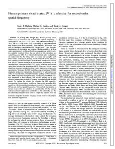
Figure 3.2: Existence curves for a single bump traveling pulse solution of equation (3.1) in the case of a homogeneous network with an exponential weight distribution W (x) = e−|x|/2 . (Left): Existence curves in the (α,a) plane. (Right) Existence curves in the (α,c) plane. Pulses only exist for small enough α (sufficiently slow adaptation). For each parameter set, there exists a stable branch (solid) of wide/fast pulses and an unstable branch (dashed) of narrow/slow pulses. In the case κ = 0.3 the branches annihilate at a saddle-node bifurcation at a critical value αc . In the other two cases, the branches end abruptly due to the fact that the eigenvalues µ± become complex–valued [65]. See Sect. 2.3 for further exposition of these ideas. with W0 = d = 1. Numerically solving equations (3.32) and (3.33) for a and c as a function of the adaptation rate α yields the existence curves shown in Fig. 3.2. This figure illustrates the well known result that for sufficiently slow adaptation (small α) there exists a pair of traveling pulses with the fast/wide pulse stable and the slow/narrow pulse unstable [51]. Also shown in the figure is the stability of the various solution branches, which can be determined analytically using an Evans function approach [72, 20, 25, 52].
Figure 3.3: Existence curves for a single bump traveling pulse solution of equation (3.1) in the case of a homogeneous network with an exponential weight distribution W (x) = W± e−|x|/2 with W± = 1 ± ρ. (Left): Plot of wave speed c± as a function of ρ for weight amplitudes W± . Dashed curve indicates arithmetic mean of pair c± . The slower branch terminates at around ρ = 0.35 due to a saddle–node bifurcation. The faster branch terminates due to a blow–up of the pulse width. (Right): Plot of pulse width a± as a function of ρ for weight amplitudes W± . The analysis of existence in a homogeneous network also provides some insights into what happens
35
when we include a periodic modulation of the weights according to equations (3.4) and (3.6). Such a modulation induces a periodic variation in the amplitude W0 of the exponential weight distribution (3.5) between the limiting values W± = (1 ± ρ)W0 . This suggests that the speed of a wave in the inhomogeneous network will be bounded by the speeds c± of a traveling wave in the corresponding homogeneous network obtained by taking W0 → W± . Note that rescaling the weight distribution in equations (3.32) and (3.33) is equivalent to rescaling the threshold according to κ → κ/(1 ± ρ). In Fig. 3.3 we plot the speeds c± and the corresponding pulse widths a± as a function of ρ. For sufficiently small ρ, the wave speed c+ increases with ρ at approximately the same rate as c− decreases so that their arithmetic mean remains constant. Therefore, one might expect that a periodic variation in weights would lead to a corresponding periodic variation in wave speed such that the mean wave speed is approximately independent of ρ. However, when a pulse enters a region of enhanced synaptic weights, the resulting increase in wave speed coincides with a rapid increase in pulse width as a function of ρ. Thus, the pulse will tend to extend into neighboring regions of reduced synaptic weights and the resulting spatial averaging will counteract the speeding up of the wave. On the other hand, when a pulse enters a region of reduced synaptic weights, the reduction in wave speed coincides with a reduction in pulse width so that spatial averaging can no longer be carried out as effectively. (The effectiveness of spatial averaging will depend on the ratio of the pulse width a to the periodicity 2πε of the weight modulation). Hence, we expect regions where the weights are reduced to have more effect on wave propagation than regions where the weights are enhanced, suggesting that a periodic weight modulation leads to slower, narrower waves. This is indeed found to be the case, both in our perturbation analysis (see Sect. 3.3.2) and our numerical simulations (see Sect. 3.4). Interestingly, we also find that traveling waves persist for larger values of ρ than predicted by our analysis of single bumps in homogeneous networks, although such waves tend to consist of multiple bumps (see Sect. 3.4).
3.3.2
Inhomogeneous network with Heaviside nonlinearity
Suppose that the homogeneous network with a Heaviside nonlinearity supports a stable traveling wave solution (U (ξ), V (ξ))T of wave speed c. As shown in Section 3.3.1, a stable/unstable pair of traveling waves exists for sufficiently slow adaptation. In order to calculate the average wave speed c¯ for nonzero ε and ρ, see equation (3.23), we first need to compute the null-vector (A(ξ), B(ξ))T of the adjoint operator L∗ defined
36
by equation (3.18). In the case of a Heaviside nonlinearity,
−c
Z ∞ dA(ξ) δ(ξ) W (ξ − ξ 0 )A(ξ 0 )dξ 0 − A(ξ) + B(ξ) + 0 dξ |U (0)| −∞ Z δ(ξ + a) ∞ + 0 W (ξ − ξ 0 )A(ξ 0 )dξ 0 = 0 |U (−a)| −∞ c dB(ξ) − − βA(ξ) − B(ξ) = 0. α dξ
(3.34)
For ξ 6= 0, −a, this has solutions of the form (A(ξ), B(ξ)T ) = ue−λξ with associated characteristic equation Mu = cλu and −1 . α
1 M= βα
(3.35)
The eigenvalues are λ = µ± = m± /c with m± given by equation (3.27). The corresponding eigenvectors are u±
=
1 1 − m±
.
(3.36)
The presence of the Dirac delta functions at ξ = 0, −a then suggests that we take the null solution to be of the form
V∗ (ξ)
=
h i γ+ u+ e−µ+ ξ Θ(ξ) + χe−µ+ (ξ+a) Θ(ξ + a) h i +γ− u− e−µ− ξ Θ(ξ) + χe−µ− (ξ+a) Θ(ξ + a)
(3.37)
with the coefficients γ± chosen such that the Dirac delta function terms that come from differentiating the null vector only appear in the A(ξ) term, γ+ u+ + γ− u−
Γ = , 0
(3.38)
and χ is a constant yet to be determined. Taking
γ±
=
±(1 − m∓ )
37
(3.39)
we have Γ = m+ − m− . In order to determine χ, substitute equation (3.37) into equation (3.34) to obtain the pair of equations 1
c(m+ − m− )
=
χc(m+ − m− )
=
|U 0 (0)|
(Λ(0) + χΛ(−a))
(3.40)
and 1 (Λ(a) + χΛ(0)) |U 0 (−a)|
(3.41)
with Z Λ(ζ)
=
∞
[(1 − m− )W (ξ + ζ)e−µ+ ξ − (1 − m+ )W (ξ + ζ)e−µ− ξ ]dξ.
(3.42)
0
We require that equations (3.40) and (3.41) are consistent with the formula for U 0 (ξ) obtained by differentiating equation (3.30) with respect to ξ:
U 0 (ξ)
=
1 − m− c(m+ − m− )
∞
Z
1 − m+ − c(m+ − m− )
0
eµ+ (ξ−ξ ) [W (ξ 0 + a) − W (ξ 0 )]dξ 0
ξ
Z
∞
0
eµ− (ξ−ξ ) [W (ξ 0 + a) − W (ξ 0 )]dξ 0 .
(3.43)
ξ
It follows that
|U 0 (0)| = −U 0 (0) =
Λ(0) − Λ(a) Λ(0) − Λ(−a) , |U 0 (−a)| = U 0 (−a) = , c(m+ − m− ) c(m+ − m− )
which, together with equations (3.40) and (3.41), implies
Λ(0) − Λ(a) = Λ(0) + χΛ(−a), χ(Λ(0) − Λ(−a)) = Λ(a) + χΛ(0).
Hence, equation (3.37) is a solution provided that
χ = −
Λ(a) . Λ(−a)
(3.44)
This is also a constructive proof that the adjoint linear operator L∗ for a Heaviside nonlinearity has a one-dimensional nullspace spanned by V∗ .
38
Having found the null solution (3.37), we now determine the phase function Φ1 given by equation (3.22) with f = H. First, the constant K of equation (3.20) is evaluated by substituting for (A(ξ), B(ξ)) using equation (3.37) and substituting for (U (ξ), V (ξ) using equations (3.30) and (3.31). The rather lengthy expression for K is given in the appendix. Next, we evaluate the double integral on the right–hand side of equation (3.22) by setting D(x) = eix and using Fourier transforms. This gives
KΦ1
where
∗
� � φ = ε
i iφ/ε e ε
Z
∞
�Z
∞
� dq e∗ (q)f] eiqx A (U )(q + ε−1 ) dx, 2π −∞
W (x) −∞
(3.45)
denotes complex conjugate and Z
∞
eiqx A(x)dx.
e = A(q)
(3.46)
−∞
In the case of a Heaviside nonlinearity and a pulse of width a, f (U (ξ)) = Θ(ξ + a) − Θ(ξ), and A(x) is given explicitly by the first component of the null vector in equation (3.37). Taking Fourier transforms of these expressions shows that
e = − 1 + χe−iqa A(q)
�
�
� γ− γ+ + , iq − µ+ iq − µ−
1 − e−iqa f] (U )(q) = iq − 0+
(3.47)
If these Fourier transforms are now substituted into equation (3.45), we have � � φ KΦ1 = ε
∞
"Z
∞
(
−1
γ+ (1 − e−i(q+ε )a + χeiqa − χe−ia/ε )eiqx W (x) (q + ε−1 + i0+ )(q − iµ+ ) −∞ −∞ ) # −1 γ− (1 − e−i(q+ε )a + χeiqa − χe−ia/ε )eiqx dq + dx. (q + ε−1 + i0+ )(q − iµ− ) 2πi
eiφ/ε ε
Z
(3.48)
The resulting integral over q can be evaluated by closing the contour in the upper half or lower-half complex q-plane depending on the sign of x, x±a. We find that there are only contributions from the poles at q = iµ± with µ± > 0, whereas there is a removable singularity at q = −ε−1 − i0+ . Thus � � φ KΦ1 = ε
h� � i γ+ eiφ/ε −ia/ε b b + (−a) − e−ia/ε Ω b + (a) 1 − χe Ω (0) + χ Ω + ε(ε−1 + iµ+ ) h� � i γ− eiφ/ε −ia/ε b b − (−a) − e−ia/ε Ω b − (a) , 1 − χe Ω (0) + χ Ω − ε(ε−1 + iµ− ) (3.49)
39
with Z b ± (s) = Ω
∞
W (x + s)e−µ± x dx
(3.50)
0
Taking the imaginary part of the above equation then determines the phase function KΦ1 for D(x) = ρ sin(x). After a straightforward calculation, we find that K φ Φ1 ( ) ρ ε
� � � � φ φ−a = (Ξ+ + Ξ− ) sin + (Π+ + Π− ) sin + ε ε � � � � φ φ−a (Υ+ + Υ− ) cos + (Ψ+ + Ψ− ) cos ε ε
(3.51)
where the explicit expressions for Ξ± , Π± , Υ± , Ψ± are given in the appendix.
Figure 3.4: (Left): Average wave speed c¯ vs. ε for various values of the modulation amplitude ρ. Critical value of ε for wave propagation failure decreases as ρ increases. (Right): Average wave speed c¯ vs. ρ for various values of the modulation period ε. For the sake of comparison, the speed curves previously plotted in Fig. 3.3 for a homogeneous network are also shown (gray curves). Other parameters are κ = 0.2, α = 0.04 and β = 2.0. Finally, we numerically calculate the average wave speed c¯ by substituting equation (3.51) into equation (3.23). Note that we use the exact expression for Φ1 that includes all higher–order terms in ε, rather than keeping only the O(1) term, since this gives a better estimate of the wave speed. In Fig. 3.4 we show some example plots of c¯ as a function of ε and ρ. It can be seen that for each choice of parameters, c¯ is a monotonically decreasing function of ε and ρ, with c¯ approaching the speed c of the homogeneous wave in the limits ε → 0 and ρ → 0. Hence, although the periodic modulation enhances the strength of connections in some regions and reduces them in others compared to the homogeneous case, see Fig. 3.1, the net result is an effective reduction in wave speed. This is consistent with our discussion of Fig. 3.3 in Section 3.3.1, where we used a spatial averaging argument combined with the observation that faster waves are wider to infer that regions of reduced synaptic weights affect wave propagation more than regions of enhanced weights. 40
Fig. 3.4 also suggests that for sufficiently small ε there exists a traveling wave solution for all ρ, 0 ≤ ρ < 1, whereas for larger values of ε there is a critical value ρc beyond which propagation failure occurs. That is, c¯ → 0 as ρ → ρc , and this critical value decreases as the periodicity ε of the inhomogeneity increases. Similarly, for sufficiently large ρ there exists a critical period εc such that c¯ → 0 as ε → εc . Analogous results were previously obtained for traveling fronts in a scalar equation [11]. It is important to bear in mind that the calculation of c¯ is based on the O(ε) perturbation analysis of Section 3.2, although we do include higher-order terms in the calculation of Φ1 . This raises the important question as to whether or not our analysis correctly predicts wave propagation failure in the full system, given that c¯ tends to approach zero at relatively large values of ε and ρ. Moreover, the perturbation analysis does not determine the stability of the wave so that propagation failure could occur due to destabilization of the wave for ρ < ρc or ε < εc . This will indeed turn out to be the case as we show in Section 3.4, where we present numerical solutions of equation (3.1) and provide further insights into the mechanism for propagation failure.
3.3.3
Smooth nonlinearities and higher–order corrections
e In the case of smooth nonlinearities, the Fourier transforms A(q) and f] (U )(q) appearing in equation (3.45) no longer have simple poles and in general Φ1 will consist of exponentially small terms. It follows that Φ1 may be less significant than the O(ε2 ) terms ignored in the perturbation expansion of (3.10). Therefore, following the treatment of traveling fronts [11], we carry out a perturbation expansion of system (3.10) to O(ε2 ). This yields an equation for (u2 , v2 ) of the form
u (ξ, τ ) ∂ 2 − + L ∂τ v2 (ξ, τ )/α v2 (ξ, τ ) u2 (ξ, τ )
= −φ02 (τ ) −φ01 (τ )
U 0 (ξ) 0
V (ξ)/α u01 (ξ)
(3.52)
h2 (ξ, + v10 (ξ)/α 0
φ ε)
where L is defined by equation (3.15) and
h2 (ξ,
φ ) ε
1 2 Z
Z
∞
W (ξ − ξ 0 )f 00 (U (ξ 0 ))[u1 (ξ 0 )]2 dξ 0 � 0 � [ξ + φ] − D W 0 (ξ − ξ 0 )f 0 (U (ξ 0 ))u1 (ξ 0 )dξ 0 ε −∞ � Z ∞ � 0 [ξ + φ] + D W (ξ − ξ 0 )[f 0 (U (ξ 0 ))u01 (ξ 0 ) + f 00 (U (ξ 0 ))U 0 (ξ 0 )u1 (ξ)]dξ 0 . ε −∞
= −
−∞ ∞
41
(3.53)
The existence of a bounded solution requires the solvability conditions (3.19) and Z
∞
φ )dξ, ε
(3.54)
∂v1 (ξ, τ ) ∂u1 (ξ, τ ) + α−1 B(ξ) ]dξ. ∂ξ ∂ξ
(3.55)
Kφ02 (τ ) + L(τ )φ01 (τ )
A(ξ)h2 (ξ,
= −∞
where Z
∞
L(τ ) =
[A(ξ) −∞
In order to evaluate the solvability condition (3.54), we must first determine u1 (ξ, φ/ε) from equation (3.14). If we choose D(x) to be a sinusoid, then u1 (ξ, φ/ε) will include terms that are proportional to sin(φ/ε) and cos(φ/ε). Thus substituting u1 (ξ/φ/ε) into equation (3.53), will generate terms of the form sin2 (φ/ε) and cos2 (φ/ε) due to the quadratic term in u1 . Using the identities 2 sin2 (x) = 1 − cos(2x) and 2 cos2 (x) = 1 + cos(2x), implies that there will be an ε-independent contribution to φ02 . Thus for smooth nonlinearities, we find that � � dφ φ 2 = c + ε C2 (c) + D2 c, , dτ ε
(3.56)
where C2 is independent of ε and D2 is exponentially small in ε. Equation (3.56) is the second–order version of the phase equation (3.21) in cases where the first–order term is exponentially small. Again the condition for wave propagation failure is that the right–hand side of equation (3.56) vanishes for some φ.
3.4
Numerical results
Our perturbation analysis suggests that as ρ increases, the mean speed of a traveling pulse decreases, and, at least for sufficiently large periods ε of the weight modulation, wave propagation failure can occur. However, one of the simplifying assumptions of our analysis is that the perturbed solution is still a traveling pulse, that is, at each time t there is a single bounded interval over which the solution is above threshold, which is equal to the pulse width a of the homogeneous pulse in the limit ε → 0. The inclusion of a periodic modulation of a monotonically decreasing weight function suggests that the assumption of a single pulse solution may break down as ρ increases towards unity. In this section we explore this issue by numerically solving the full system of equations (3.1) in the case of a Heaviside nonlinearity (f = H), and show that wave propagation can persist in the presence of multiple bumps. Numerical simulations of propagating pulses are
42
Figure 3.5: (Top Left): Stable traveling pulse for a homogeneous network with exponential weight function (3.5) and fixed parameters κ = 0.2, β = 2.0, and α = 0.04 (for all plots). (Top Right): Corresponding traveling pulse for an inhomogeneous network with weight distribution (3.4) and a sinusoidal modulation with ε = 0.1 and ρ = 0.3. We see rippling in the interior of the pulse. (Bottom Left): Using a more severe inhomogeneity, ρ = 0.8, leads to rippling in the active region of the pulse such that now the interior crosses below threshold periodically. (Bottom Right): For ρ = 1, the effect is even more severe.
43
Figure 3.6: (Top Left): Comparison of the wave profiles at time t = 10 for the homogeneous (dashed line) and the inhomogeneous (solid line) cases. Here, parameters are κ = 0.2, β = 2.0, α = 0.04, ε = 0.3, and ρ = 0.3. Including periodic modulation clearly thins the pulse as we see its profile fits within that of the homogeneous medium. (Top Right): Subtraction of the homogeneous solution from the inhomogeneous at time t = 10. We see here an approximation of u1 (x, t), from our perturbation analysis. The dominant detail is the oscillations with period 2πε. (Bottom Left): Profile comparison at t = 200. Homogeneous solution has moved well ahead of the inhomogeneous due to speed difference. (Bottom Right): Pseudocolor plot of u1 (x, t), obtained by subtracting the homogeneous solution from the inhomogeneous. The dark bands delineate the underlying homogeneous solution.
44
Figure 3.7: A collection of traveling wave profiles taken at time t = 10 for various amplitudes ρ and ε = 0.1. Other parameters as in Fig. 3.5. (Top Left): ρ = 0.1. Notice that rippling of the activity does not dip below threshold within the pulse interior. (Top Right): ρ = 0.3. Rippling crosses below threshold at the edges of the pulse creating a couple of bumps. (Bottom Left): ρ = 0.7. Rippling now generates a multiple bump solution. (Bottom Right): ρ = 0.8. carried out using MATLAB. Initial conditions are taken to be solutions to the homogeneous problem given by equations (3.30) and (3.31). We then apply backward Euler to the linear terms, and forward Euler with a Riemann sum for the convolution operator. Space and time discretizations are taken to be ∆t = 0.01 and ∆x = 0.01. The numerical results are stable with respect to reductions in the mesh size provided that ∆x � 2πε. Finally, boundary points evolve freely, rather than by prescription, and the domain size is wide enough so that pulses are unaffected by boundaries. In Fig. 3.5 we show some examples of traveling pulse solutions in an inhomogeneous network with weight distribution given by equations (3.4), (3.5) and (3.6). The period of the modulation is taken to be relatively small (ε = 0.1). We take as initial conditions the invariant profile for the corresponding homogeneous case,
45
Figure 3.8: A series of snapshots in time of a traveling pulse for κ = 0.2, β = 2.0, α = 0.04, ρ = 0.3, ε = 0.3. The interior of the pulse consists of non-propagating, transient ripples. The disappearance of ripples at one end and the emergence of new ripples at the other end generates the propagation of activity. Notice that the solitary wave profile is not invariant, reflecting the underlying inhomogeneity. (Top Left): t = 1 (Top Right): t = 5 (Bottom Left): t = 10. (Bottom Right): t = 20.
46
obtained by solving in traveling wave coordinates for the ε = 0 case, which gives (U, V ) in equations (3.30) and (3.31). It can be seen from Fig. 3.5 that as the amplitude ρ of the periodic modulation increases the wave slows down and narrows, which is consistent with our perturbation analysis. Moreover, the network activity develops a rippling within the interior of the pulse as can be seen more clearly in Fig. 3.6, where we directly compare the numerical solution of the homogeneous network with that of a corresponding inhomogeneous network. Superimposing the two wave profiles at an early time (t = 10) illustrates the thinning of the pulse, and shows that the difference of the two wave profiles is an oscillatory component of approximately zero mean, which would correspond to u1 in our perturbation analysis. Similarly, comparing the two wave profiles at a later time (t = 200) illustrates the slowing down of the pulse. As ρ increases the amplitude of the ripples also increases such that for sufficiently large ρ, activity at any given time t alternates between superthreshold and subthreshold domains. This is illustrated in Fig. 3.7. A closer look at the time evolution of the wave profile when the rippling is above threshold within the interior of the pulse shows that individual ripples are non-propagating and transient, with new ripples appearing at the leading edge of the wave and subsequently disappearing at the trailing edge, see Fig. 3.8. Interestingly, such behavior persists for large ρ when the ripples cross below threshold within the interior of the pulse, see Fig. 3.9. Now the pulse actually consists of multiple bumps, each of which is non-propagating but only exists for a finite length of time. The sequence of events associated with the emergence and disappearance of these bumps generates a wave envelope that behaves very much like a single coherent traveling pulse. Hence, for sufficiently short wavelength oscillatory modulations of the weight distribution, the transient multiple bump solution can be homogenized and treated as a single traveling pulse. However, the wave speed of the multiple bump solution differs from that predicted using perturbation theory. This is shown in Fig. 3.10, where we compare the c¯ vs. ε curves obtained using perturbation theory with data obtained by directly simulating the full system (3.1). In the case of small ρ, a stable (single bump) traveling pulse persists for all ε, 0 ≤ ε < 1 and c¯ is a monotonically decreasing function of ε. Moreover, the numerically calculated value of the average wave speed agrees quite well with the first-order perturbation analysis. On the other hand, for large values of ρ, such agreement no longer holds, and we find that the traveling pulse destabilizes at a critical value of ε that is well below the value predicted from the perturbation analysis. In Fig. 3.11 we compare the behavior of traveling pulses for short wavelength (ε = 0.2) and long wavelength (ε = 0.9) periodic modulation. The amplitude is taken to be relatively large, ρ = 0.8, so that multiple bump solutions occur. We see that for long wavelength modulation, the initial pulse transitions into a non–propagating multiple bump solution, with successive bumps disappearing sequentially and no
47
Figure 3.9: A series of snapshots in time of the “pulse” profile for κ = 0.2, β = 2.0, α = 0.04, ρ = 0.8, ε = 0.3. The solitary pulse corresponds to the envelope of a multiple bump solution, in which individual bumps are non-propagating and transient. The disappearance of bumps at one end and the emergence of new bumps at the other end generates the propagation of activity. Notice that the solitary wave profile is not invariant, reflecting the underlying inhomogeneity. (Top Left): t = 10 (Top Right): t = 15 (Bottom Left): t = 20. (Bottom Right): t = 30.
48
Figure 3.10: Comparison of perturbation theory with direct numerical simulations. Continuous curves show average wave speed c¯ as a function of ε obtained using perturbation theory. Data points are the corresponding wave speeds determined from numerically solving equation (3.1). In the case of low amplitude modulation (ρ = 0.3, dark curve) a stable traveling pulse persists for all ε, ε < 1, whereas for large amplitude modulation (ρ = 0.8, light curve), wave propagation failure occurs as ε increases. additional bumps being created; the failure to generate new bumps means that activity cannot propagate. We can see this more clearly when examining a series of snapshots of the pulse/bump profiles in Fig. 3.12. In conclusion, one way to understand wave propagation failure for large ρ is to note that a large amplitude periodic weight modulation can generate a pinned multiple bump solution. However, in the absence of any inhibition such a multiple bump solution is unstable [40, 60]. In the case of small ε, destabilization of the bumps generates new bumps at the leading edge of the bump such that activity can propagate in a coherent fashion. Increasing ε prevents the creation of new bumps and propagation failure occurs. The effect of the periodic weight modulation on a different type of solution is illustrated in Fig. 3.13, where, motivated by a prior numerical study of multiple bumps [40], the initial condition of the network is taken to consist of three bumps,
u(x, 0) =
1 X j=−1
cos
�x� ε
� exp −
0.1(x − j · 20) ε
�2 ! .
(3.57)
Each initial bump generates a pair of left and right moving fronts. In the homogeneous case, we see that collision of left and right moving waves results in a bidirectional front. That is, the region within the interior
49
Figure 3.11: Comparison of traveling pulses in the case of short and long wavelength periodic modulation with ρ = 0.8 and all other parameters as in Fig. 3.5. (Left): For short wavelength modulation (ε = 0.2) the traveling pulse shrinks and slows, but does not annihilate. (Right): For long wavelength modulation (ε = 0.9) wave propagation failure occurs. The initial pulse transitions into a collection of multiple equal width stationary bumps which are unstable. of the boundary formed by the two outermost fronts becomes superthreshold. In the inhomogeneous case, the collision of the waves is insufficient to maintain activity across this region, and one finds a pair of counterpropagating pulses.
3.5
Discussion
In this chapter we analyzed wave propagation in an excitatory neural network treated as a periodic excitable medium. The periodicity was introduced as an inhomogeneous periodic modulation in the long-range synaptic connections, and was motivated by the existence of patchy horizontal connections in cerebral cortex. We showed that for small amplitude, short wavelength periodic modulation the main affect of the inhomogeneity is to slow down a traveling pulse, and the mean speed of the pulse can be estimated quite well using perturbation theory. In the case of large amplitude modulation, a stable traveling pulse still exists for sufficiently small ε, but now the pulse is the envelope of a multiple bump solution in which individual bumps are unstable and transient. Wave propagation arises via the appearance (disappearance) of bumps at the leading (trailing) edge of the pulse. As ε increases wave propagation failure occurs due to the fact that there is insufficient activity to generate new bumps. Although the existence of multiple bump traveling “pulses” is interesting from a dynamical systems perspective, it is less clear whether such solutions can be observed in real neural tissue. Further experiments
50
Figure 3.12: A series of snapshots in time of the “pulse” profile for the inhomogeneous network with κ = 0.2, β = 2.0, α = 0.04, ρ = 0.8, ε = 0.9. (Top Left): The initial wave profile, which is taken to be the invariant wave profile U of the homogeneous network. (Top Right): Shortly after the simulation begins (t = 0.5), the interior of the pulse develops ripples such that the active region contains a subregion for which activity is subthreshold. (Bottom Left): At time t = 2 a multiple bump profile has emerged. We can really see here how a multiple bump solution, as defined by multiple neighboring standing profiles, emerges from the pulse profile of t = 0. (Bottom Right): Collapse of the pulse interior occurs due to the disappearance of the unstable bumps. Since no new bumps emerge, there is no propagating activity.
51
Figure 3.13: (Left): In the case of a homogeneous network, a three bump initial condition evolves into a bidirectional front following the collision of left and right traveling waves. Parameters are κ = 0.2, β = 2.0, α = 0.04. (Right): In the corresponding inhomogeneous network with ε = 0.2 and ρ = 0.8, the collision of left and right traveling waves results in a pair of counterpropagating pulses. Here the modulated synaptic interactions are insufficient to maintain activity in the region between the two pulses. in cortical slice or in vivo as described in Section 2.1 may reveal similar phenomena. One of the biological limitations of the integro-differential equations used in this and other studies is that although these equations support traveling waves that have speeds consistent with neurophysiology, the pulses tend to be too wide. That is, taking the range of synaptic connections to be 1mm, the width of a stable pulse tends to vary between 5 − 30mm, see Fig. 3.2, whereas waves in slices tend to be only 1mm wide [51]. More realistic widths and wave speeds could be generated by taking the effective range of synaptic connections to be a few hundred µm (as described in Sect. 1.2), that is, by assuming that the predominant contribution to synaptic excitability is via local circuitry rather than via long–range patchy horizontal connections. However, inhomogeneities occurring at smaller spatial scales are unlikely to exhibit any periodic structure. Irrespective of these particular issues, our analysis raises a more general point that would be interesting to pursue experimentally, namely, is it possible to detect the effects of network inhomogeneities by measuring the properties of traveling waves? Signatures of such inhomogeneities would include time–dependent rippling of the wave profile and variations in wave speed. However, such features may not be detectable given the current resolution of microelectrode recordings.
52
Chapter 4
Future directions: Applying the coupled hypercolumn model to visual percepts In this chapter, we discuss how we shall model two visual percepts: (i) contour integration, the visual cortex’s apparent binding together of edges, contours, and textures as distinct objects; and (ii) binocular rivalry, the brain perceiving the alternation between two different images presented to either eye. We suggest that these processes may be modeled by a coupled hypercolumn model, wherein cortical hypercolumns containing neurons with a full range of orientation preferences are connected via long range connections. We describe this model in detail in Section 1.3.
4.1
Contour saliency with the coupled hypercolumn model
We can use the coupled ring model to study how the primary visual cortex may accomplish the task of grouping a contour presented in visual space as explained in Section 2.2. Due to the feature specific nature of horizontal connections, theoretically, an initial blip of attentionally increased firing rate could spread along horizontal connections, guided by the already excited neurons containing the rest of the contour in their RFs (see Fig. 2.2). Therefore, using such equations as (1.7), we can study the effect of perturbing the excited steady state at one point in visual space. Whether or not such a perturbation spreads along the line of input
53
hl (ri , φ) or not may suggest whether or not the mechanism of horizontal connections is a viable substrate for contour saliency. The coupled ring model is a major reduction of the true functional architecture of the visual cortex, but it captures some general properties of orientation specificity, distinct patches, and two space scales of synaptic connections. Macaques’ horizontal connections do not possess the same anisotropy ideal for collinear binding as tree shrews and new world monkeys; thus, theirs and humans’ brains may perceptually group using feedback connections. Nonetheless, visual processing of contours may be simplistically modeled by rings, containing neurons specific to the full range of orientation preferences, connected by collinear synaptic weighting. As a first attempt at understanding contour tracing, we analyze the coupled hypercolumn model when a horizontal line is given as visual input. Therefore, two-dimensions can be collapsed to one dimension. We then relabel the activity ul (ri , φ, t) in orientation φ cells in the ith ring at time t with a single index i, rather than with a spatial location. Also, rather than using both excitatory and inhibitory populations, we use one population of neurons with a Mexican hat connectivity. Therefore, these model neurons excite cells close to them and inhibit cells farther away. They also possess horizontal connections to iso-orientation patches in neighboring rings with collinear properties as discussed. Thus, activity need no longer be indexed by l = E, I, since there is only one type of “neuron.” We then write the integro-differential equation for activity in an iso-orientation patch in the ith ring as ∂ui (φ, t) ∂t
=
−ui (φ, t) + hi (φ) +
N Z X j=1
π/2
wi,j (φ|φ0 ) ∗ f (uj (φ0 , t))
−π/2
dφ0 π
(4.1)
We thus consider the weight function to have the form
wi,j (φ|φ0 )
=
W (φ − φ0 )δi,j + εw ˆi,j (φ|φ0 )(1 − δi,j ),
(4.2)
and
W (x) = γE e−x
2
/s2E
− γI e−x
2
/s2I
,
(4.3)
where γE , γI are relative strengths of local synaptic excitation and inhibition, respectively, and sE , sI are the spatial constants for the excitation and inhibition Gaussians. The weight function w ˆi,j (φ|φ0 ) should be some function that decays with cortical distance and couples φ patches most strongly to other φ0 patches of
54
like orientation, as discussed. We consider the input from LGN to be
hi (φ)
=
C cos(2φ),
(4.4)
where C > 0 is the contrast of the line. Since the input is horizontal, it should be strongest to the neurons that prefer φ = 0 stimuli. We ignore the activity of neurons not receiving input. Analysis of how the single hypercolumn possesses sharp orientation tuning was carried out in a previous study [12]. Therefore, we plan to carry out a study of how a perturbation of the active steady state within one hypercolumn’s activity (say u1 (φ, t)) spreads to the other hypercolumns. We will exploit the fact that horizontal connections are weak relative to local circuitry and use bifurcation analysis to derive dynamical equations for excited modes close to the bifurcation point. In doing so, the system of integrodifferential equations should reduce to a system of ordinary differential equations called amplitude equations. Such amplitude equations represent the evolution of overall activity in each ring. If indeed the amplitude equations imply that the initial activity blip propagates sequentially along rings, this implies that horizontal connections may be a feasible mechanism for contour saliency. Of course, not all contours are straight lines. Therefore, it will be necessary to pursue similar analysis under the assumption that input from the LGN is a circle of certain curvature. The question then arises as to how much curvature a circle may have an still be integrated by this process of a spreading attentional blip. The problem may still be reduced from two dimensions to one, since we can consider only the rings whose RFs contain the stimulus. If indeed the propagation fails for a certain amount of curvature, this may imply that perceptual grouping of high curvature stimuli may need to recruit higher order processes such as feedback or RF widening in V2 and V4. As this project develops, many more interesting questions should arise.
4.2
Binocular rivalry in the coupled hypercolumn model
Presumably, the neural substrate for binocular rivalry, as described in Section 2.2, should be that the two groups of neurons representing either rival figure should trade off having the highest firing rate. Reciprocal inhibition mechanisms are often used to describe this phenomenon. The dominant eye neurons strongly inhibit the competing neurons, suppressing them. Computational models often use some slow negative feedback process, such as spike frequency adaptation to reduce the firing rate of the dominant population so that the suppressed population can eventually become active [61]. Wilson uses a two-stage competitive 55
model, which includes a monocular and binocular level of neurons [68]. In doing so, he is able to capture the quantitative effect of the period of eye dominance decreasing as the stimulus strength increases. On the other hand, Rinzel and his colleagues consider a noise-driven attractor model, wherein switching between eyes requires inherent noise [48]. They derive a rate-based mean field model using energy methods. By sending information about the dominant eye’s stimulus to the competing eye, the activity level of the competing eye is reduced by inhibition. The mean field model is extended to a spiking neuronal attractor network, wherein similar results hold. Thus, previous modeling studies employ computational models, which are difficult to study analytically. We wish to address binocular rivalry using a hypercolumn model of the type described in Section 1.3. It would be interesting to use a single ring of the full spectrum of orientation preferences to model this oscillation in elevated firing rate. With the inclusion of excitatory and inhibitory cells, the activity in the neural field could capture the experimentally observed phenomenon. Basically, two different gratings of different orientation would be presented as input to the ring. Since connections from both excited populations would inhibit the activity of the other, the two would compete for the most elevated firing rate. Decay of activity would eventually reduce the firing rate of the winning population and the other population would be resultantly disinhibited. Of course, the specifics of the mathematical analysis are not yet apparent, but by reducing the neural field integro-differential equations to a system of amplitude equations, one could analyze the stability of either state dependent on the stimuli. Such a project is intimately related to modeling contour saliency as elevated firing rate in the ring model represents the dominant percept. Also, horizontal connections via collinearity are essential for the physiological accomplishment of this task. We would then extend the results for binocular rivalry in the single ring to multiple rings. Annular stimuli as used by Wilson and colleagues would require multiple hypercolumns. Switching between perception of either stimulus would be initiated in a single ring. Coupling between rings would cause the switch to propagate along horizontal connections joining rings until the entire network of hypercolumns was switched. We could analyze this process using the type of amplitude equation approach similar to the contour integration problem.
56
Appendix In this appendix we present the explicit parameter-dependent expressions for the various coefficients appearing in the solution of the phase function Φ1 , equation (3.19). First, the constants premultiplying the periodic functions on the right hand side of equation (3.19) are as follows:
Ξ±
=
Π±
=
Υ±
=
Ψ±
=
� � �� γ± χ e−a − e−µ± a e−µ± 1 + + 1 + µ2± ε2 2(1 + µ± ) 2 µ± − 1 µ± + 1 � � e−a γ± χ − − 1 + µ2± ε2 2(1 + µ± ) 2(µ± + 1) � � �� γ± χµ± ε e−a − e−µ± a e−µ± a µ± ε − + − 1 + µ2± ε2 2(1 + µ± ) 2 µ± − 1 µ± + 1 � � −a γ± µ± εe χµ± ε + . 1 + µ2± ε2 2(1 + µ± ) 2(1 + µ± )
Second, the constant scaling factor K on the left-hand side of equation (3.19) is determined by substituting equations (3.30), (3.31) and (3.37) into equation (3.20). Using the fact that the null vector is zero for ξ < −a, we can expand the integral out in terms of definite integrals of exponential products with the
57
M± (ξ) functions:
K
=
Z
∞
e−µ+ ξ M0+ (ξ)dξ Z ∞ +[γ− (1 − m− )(1 + χe−µ− a )(1 + α−1 β −1 (m+ − 1)(1 − m− ))] e−µ− ξ M0+ (ξ)dξ 0 Z ∞ −µ+ a −1 −1 −[γ+ (1 − m+ )(1 + χe )(1 + α β (m− − 1)(1 − m+ ))] e−µ+ ξ M0− (ξ)dξ 0 Z ∞ e−µ− ξ M0− (ξ)dξ −[γ− (1 − m+ )(1 + χe−µ− a )(1 − α−1 β −1 (1 − m− )2 )]
[γ+ (1 − m− )(1 + χe−µ+ a )(1 − α−1 β −1 (1 − m+ )2 )]
0
0
+χ[γ+ e−µ+ a (1 − m− )(1 − α−1 β −1 (1 − m+ )2 )]
0
Z
e−µ+ ξ M0+ (ξ)dξ
−a
+χ[γ− e−µ− a (1 − m− )(1 + α−1 β −1 (m+ − 1)(1 − m− ))] −χ[γ+ e−µ+ a (1 − m+ )(1 + α−1 β −1 (m− − 1)(1 − m+ ))]
Z
0
−a Z 0
e−µ− ξ M0+ (ξ)dξ e−µ+ ξ M0− (ξ)dξ
−a
−χ[γ− e−µ− a (1 − m+ )(1 − α−1 β −1 (1 − m− )2 )]
Z
0
e−µ− ξ M0− (ξ)dξ
−a
The individual integrals can be computed as follows: ∞
e−a − 1 2c(m+ − m− )(µ± + 1)2 0 Z ∞ e−a − 1 e−µ+ ξ M0− (ξ)dξ = 2c(m+ − m− )(µ− + 1)(µ+ + 1) 0 Z ∞ e−a − 1 e−µ− ξ M0+ (ξ)dξ = 2c(m+ − m− )(µ+ + 1)(µ− + 1) 0
Z
e−µ± ξ M0± (ξ)dξ =
and 0
Z
e−µ± a M0± (ξ)dξ
=
e−µ+ ξ M0− (ξ)dξ
=
e−µ− ξ M0+ (ξ)dξ
=
−a
Z
0
−a
Z
0
−a
a 1 − e(µ± −1)a + µ± − 1 (µ± − 1)2 � a e−a (e(µ± +1)a − 1) + − (µ± + 1)2 2(µ± + 1) � 1 1 − e−(µ− −µ+ )a e(µ+ −1)a − 1 − 2c(m+ − m− ) (µ− − µ+ )(µ− − 1) (µ+ − 1)(µ− − 1) � eµ+ a − e−a 1 − e−(µ− −µ+ )a + − (µ+ + 1)(µ− + 1) (µ− + 1)(µ− − µ+ ) � 1 − e−(µ+ −µ− )a e(µ− −1)a − 1 1 − 2c(m+ − m− ) (µ − 1)(µ+ − µ− ) (µ+ − 1)(µ− − 1) � e(µ− +1)a − 1 1 − e−(µ+ −µ− )a −a +e − . (µ+ + 1)(µ− + 1) (µ+ + 1)(µ+ − µ− ) 1 2c(m+ − m− )
�
58
Bibliography [1] S. Amari. Dynamics of pattern formation in lateral inhibition type neural fields, Biol. Cybern. 27: 77-87, 1977. [2] A. Angelucci, J.B. Levitt, E.J.S. Walton, J.M. Hupe, J. Bullier, and J.S. Lund. Circuits for local and global signal integration in primary visual cortex. J. Neurosci. 22: 8633-8646, 2002. [3] A. Angelucci and P.C. Bressloff. The contribution of feedforward, lateral and feedback connections to the classical receptive field center and extra-classical receptive field surround of primate V1 neurons. Prog. Brain Res. 154: 93-121, 2006. [4] R. Ben-Yishai, R.L. Bar-Or, and H. Sompolinsky. Theory of orientation tuning in visual cortex. Proc. Natl. Acad. Sci. 92: 3844-3848, 1995. [5] A. Benucci, R.A. Frazor, and M. Carandini. Standing waves and traveling waves distinguish two circuits in visual cortex, Neuron 55: 103-117, 2007. [6] R.L. Beurle. Properties of a mass of cells capable of regenerating pulses. Philos. Trans. R Soc. Lond. B 240: 55-94, 1956. [7] R. Blake and N.K. Logothetis. Visual competition. Nat. Rev. Neurosci. 3: 1-11, 2002. [8] G.G. Blasdel. Orientation selectivity, preference, and continuity in monkey striate cortex. J. Neurosci. 12: 3139-3161, 1992. [9] W.H. Bosking, Y. Zhang, B. Schofield, and D. Fitzpatrick. Orientation selectivity and the arrangement of horizontal connections in tree shrew striate cortex, J. Neurosci. 17: 2112-2127, 1997.
59
[10] P.C. Bressloff, J.D. Cowan, M. Golubitsky, P.J. Thomas, and M. Wiener. Geometric visual hallucinations, Euclidean symmetry, and the functional architecture of striate cortex. Phil. Trans. Roy. Soc. Lond. B 356: 299-330, 2000. [11] P.C. Bressloff. Traveling fronts and wave propagation failure in an inhomogeneous neural network, Physica D 155: 83-100, 2001. [12] P.C. Bressloff and J.D. Cowan. An amplitude equation approach to contextual effects in visual cortex, Neural Comput. 14: 493-525, 2002. [13] P.C. Bressloff. Spatially periodic modulation of cortical patterns by long-range horizontal connections, Physica D, 185: 131-157, 2003. [14] P.C. Bressloff. Pattern formation in visual cortex. In Methods and Models in Neurophysics Les Houches Lectures, 2004. [15] E.M. Callaway. Local circuits in primary visual cortex of the macaque monkey. Ann. Rev. Neurosci. 21: 47-74, 1998. [16] R.D. Chervin, P.A. Pierce, and B.W. Connors. Propagation of excitation in neural network models. J. Neurophysiol. 60: 1695-1713, 1988. [17] B.W. Connors and Y. Amitai. Generation of epileptiform discharge by local circuits of neocortex. In: Epilepsy: models, mechanisms, and concepts. P.A. Schwartkroin, ed., Cambridge University Press, Cambridge, UK, pp. 388-423, 1993. [18] D. Contreras. Propagating waves in visual cortex. Neuron 55: 3-5, 2007. [19] S. Coombes. Waves, bumps, and patterns in neural field theories, Biol. Cybern. 93: 91-108, 2005. [20] S. Coombes and M.R. Owen. Evans functions for integral neural field equations with Heaviside firing rate function, SIAM J. Appl. Dynam. Syst. 3: 574-600, 2004. [21] S. Coombes and M.R. Owen. Bumps, breathers, and waves in a neural network with spike frequency adaptation, Phys. Rev. Lett. 94: 148102, 2005. [22] D.P. Edwards, K.P. Purpura, E. Kaplan. Contrast sensitivity and spatial frequency response of primate cortical neurons in and around the cytochrome oxidase blobs, Vision Res. 35: 1501-23, 1995.
60
[23] G.B. Ermentrout and J.B. McLeod. Existence and uniqueness of travelling waves for a neural network. Proc. R. Soc. Edin. 123A: 461-478, 1993. [24] G.B. Ermentrout and D. Kleinfeld. Traveling electric waves in cortex: insights from phase dynamics and speculation on a computational role. Neuron 29: 33-44, 2001. [25] S.E. Folias and P.C. Bressloff. Stimulus-locked traveling waves and breathers in an excitatory neural network, SIAM J. Appl. Math. 65: 2067-2092, 2005. [26] C.D. Gilbert and T.N. Wiesel. Columnar specificity of intrinsic horizontal and corticocortical connections in cat visual cortex. J. Neurosci. 9: 2432-2442. [27] C.D. Gilbert. Horizontal integration and cortical dynamics, Neuron 9: 1-13, 1992. [28] C.D. Gilbert and M. Sigman. Brain states: Top-down influences in sensory processing. Neuron 54: 677-696, 2007. [29] D. Golomb and Y. Amitai. Propagating neuronal discharges in neocortical slices: Computational and experimental study. J. Neurophysiol. 78: 1199-1211, 1997. [30] J. Guckenheimer and P.J. Holmes. Nonlinear Oscillations, Dynamical System and Bifurcations of Vector Fields, Springer, Berlin, 1983. [31] B.S. Gutkin, G.B. Ermentrout, J. O’Sullivan. Layer 3 patchy recurrent excitatory connections may determine the spatial organization of sustained activity in the primate prefrontal cortex, Neurocomputing 32: 391-400, 2000. [32] D.H. Hubel and T.N. Wiesel. Receptive fields and functional architecture of monkey striate cortex, J. Physiol. Lond. 195: 215-243, 1968. [33] J.P. Keener. Propagation of waves in an excitable medium with discrete related sites, SIAM J. Appl. Math. 61: 317-334, 2000. [34] J.P. Keener. Homogenization and propagation in the bistable equation, Physica D 136: 1-17, 2000. [35] Z.P. Kilpatrick, S.E. Folias, and P.C. Bressloff. Traveling pulses and wave propagation failure in inhomogeneous neural media, SIAM J. Appl. Dyn. Syst. (in press, 2008)
61
[36] D. Kleinfeld, K.R. Delaney, M.S. Fee, J.A. Flores, D.W. Tank, and A. Galperin. Dynamics of propagating waves in the olfactory network of a terrestrial mollusk: an electrical and optical study. J. Neurophysiol. 72: 1402-1419, 1994. [37] E. Kobatake and K. Tanaka. Neuronal selectivities to complex object features in the ventral visual pathway of the macaque cerebral cortex. J. Neurophysiol. 71: 856-867, 1994. [38] Y.W. Lam, L.B. Cohen, M. Wachowiak, and M.R. Zochowski. Odors elicit three different oscillations in the turtle olfactory bulb. J. Neurosci., 20:749-762, 2000. [39] J.W. Lance. Current concepts of migraine pathogenesis. Neurology, 43:11-15, 1993. [40] C.R. Laing, W.C. Troy, B.S. Gutkin, and G.B. Ermentrout. Multiple bumps in a neuronal model of working memory, SIAM J. Appl. Math. 63: 62-97, 2002. [41] C.R. Laing and W.C. Troy. Two-bump solutions of Amari-type models of neuronal pattern formation, Physica D 178: 190-218, 2003. [42] A.G. Leventhal, K.G. Thompson, D. Liu, Y. Zhou, S. Ault. Concomitant sensitivity to orientation, direction, and color of cells in layers 2, 3, and 4 of monkey striate cortex, J. Neurosci. 15: 1808-1818, 1995. [43] J.B. Levitt, D.A. Lewis, T. Yoshioka, and J.S. Lund. Topography of pyramidal neuron intrinsic connections in macaque prefrontal cortex, J. Comp. Neurol. 338: 360-376, 1993. [44] M. Livingstone and D. Hubel. Segregation of form, color, movement, and depth: anatomy, physiology, and perception, Science 240: 740-749, 1988. [45] D.A. Lewis and S.A. Anderson. The functional architecture of the prefrontal cortex and schizophrenia, Psychol. Med. 25: 887-894, 1995. [46] R. Malach, Y. Amir, M. Harel, and A. Grinvald. Relationship between intrinsic connections and functional architecture revealed by optical imaging and in vivo targeted bicytin injections in primate striate cortex, Proc. Natl. Acad. Sci. 90: 10469-10473, 1993. [47] D.S. Melchitzky, S.R. Sesack, M.L. Pucak, and D.A. Lewis. Synaptic targets of pyramidal neurons providing intrinsic horizontal connections in monkey prefrontal cortex, J. Comp. Neurol. 390: 211-224, 1998. 62
[48] R. Moreno-Bote, J. Rinzel, and N. Rubin. Noise-induced alternations in an attractor network model of perceptual bistability. J. Neurophysiol. 98: 1125-1139, 2007. [49] K. Obermayer and G.G. Blasdel. Geometry of orientation and ocular dominance columns in monkey striate cortex. J. Neurosci. 13: 4114-4129, 2000. [50] B.J.A. Palanca and G.C. DeAngelis. Does neural synchrony underlie visual feature grouping?, Neuron 46: 333-346, 2005. [51] D.J. Pinto and G.B. Ermentrout. Spatially structured activity in synaptically coupled neuronal networks: I. Traveling fronts and pulses, SIAM J. Appl. Math. 62: 206-225, 2001. [52] D.J. Pinto, S.L. Patrick, W.C. Huang, and B.W. Connors. Initiation, propagation, and termination of epileptiform activity in rodent neocortex in vitro involve distinct mechanisms. J. Neurosci. 25: 8131-8140, 2005. [53] D.J. Pinto, R.K. Jackson, and C.E. Wayne. Existence and stability of traveling pulses in an continuous neuronal network. SIAM J. Appl. Dyn. Syst. 4: 954-984, 2005. [54] J.C. Prechtl, L.B. Cohen, B. Pasaram, P.P. Mitra, and D. Kleinfeld. Visual stimuli induce waves of activity in turle cortex. Proc. Natl. Acad. Sci. 94: 7621-7626, 1997. [55] K.A. Richardson, S.J. Schiff, and B.J. Gluckman. Control of traveling waves in the mammalian cortex. Phys. Rev. Lett. 94: 028103, 2005. [56] K.S. Rockland and J. Lund. Intrinsic laminar lattice connections in primate visual cortex. J. Comp. Neurol. 216: 303-318, 1983. [57] P.R. Roelfsema, A.K. Engel, P. Konig, and W. Singer, Visuomotor integration is associated with zero time-lag synchronyzation among cortical areas. Nature 385: 1157-1161, 1997. [58] P.R. Roelfsema, V.A.F. Lamme, H. Spekreijse. Synchrony and covariation of firing rates in the primary visual cortex during contour grouping. Nat. Neurosci. 7: 982-991, 2004. [59] P.R. Roelfsema. Cortical algorithms for perceptual grouping. Ann. Rev. Neurosci. 29: 203-227, 2006. [60] J.E. Rubin and W.C. Troy. Sustained spatial patterns of activity in neuronal populations without recurrent excitation, SIAM J. Appl. Math. 64: 1609-1635, 2004.
63
[61] A. Shpiro, R. Curtu, J. Rinzel, and N. Rubin. Dynamical characteristics common to neuronal competition models. J. Neurophysiol. 97: 462-473, 2007. [62] L.C. Sincich and J.C. Horton. The circuitry of V1 and V2: Integration of color, form, and motion, Ann. Rev. Neurosci. 28: 303-326, 2005. [63] W. Singer and C.M. Gray. Visual feature integration and the temporal correlation hypothesis. Ann. Rev. Neurosci. 18: 555-586, 1995. [64] R.B. Tootell, M.S. Silverman, E. Switkes, and R.L. DeValois. Deoxyglucose analysis of retinotopic organization of primate striate cortex. Science 218: 902-904, 1982. [65] W.C. Troy and V. Shusterman. Patterns and features of families of traveling Waves in large-scale neuronal networks, SIAM J. Appl. Dyn. Syst. 6: 263-292, 2007. [66] J-Y. Wu, L. Guan, and Y. Tsau. Propagating activity during oscillations and evoked responses in neocortical slices. J. Neurosci. 19: 5005-5015, 1999. [67] H.R. Wilson, R. Blake, and S-H Lee. Dynamics of travelling waves in visual perception. Nature 412: 907-910, 2001. [68] H.R. Wilson. Computational evidence for a rivalry hierarchy in vision. Proc. Natl. Acad. Sci. 100: 14499-14503, 2003. [69] H.R. Wilson and J.D. Cowan. A mathematical theory of functional dynamics of cortical and thalamic nervous tissue, Kybernetik 13: 55-80, 1973. [70] W. Xu, X. Huang, K. Takagaki, and J. Wu. Compression and reflection of visually evoked cortical waves, Neuron 55: 119-129, 2007. [71] T. Yoshioka, G.G. Blasdell, J.B. Levitt, and J.S. Lund. Relation between patterns of intrinsic lateral connectivity, ocular dominance, and cytochrome oxidase-reactive regions in macaque monkey striate cortex, Cerebral Cortex 6: 297-310, 1996. [72] L. Zhang. On stability of traveling wave solutions in synaptically coupled neuronal networks, Differential Integral Equations 16: 513-536, 2003. [73] L. Zhang. Existence, uniqueness, and exponential stability of traveling wave solutions of some integral differential equations arising from neuronal networks, J. Differential Equations 197: 162-196, 2004.
64