trees, i.e. trees in which every node can have an arbitrary (but finite) number .... The tree rewriting model presented in this section is inspired by the Active XML.
Tree Pattern Rewriting Systems⋆ B. Genest3 , A. Muscholl1 , O. Serre2 , and M. Zeitoun1 1
LaBRI, Bordeaux; 2 LIAFA, Paris 7 & CNRS; 3 IRISA, Rennes 1 & CNRS
Abstract. Classical verification often uses abstraction when dealing with data. On the other hand, dynamic XML-based applications have become pervasive, for instance with the ever growing importance of web services. We define here Tree Pattern Rewriting Systems (TPRS) as an abstract model of dynamic XML-based documents. TPRS systems generate infinite transition systems, where states are unranked and unordered trees (hence possibly modeling XML documents). Their guarded transition rules are described by means of tree patterns. Our main result is that given a TPRS system (T, R), a tree pattern P and some integer k such that any reachable document from T has depth at most k, it is decidable (albeit of non elementary complexity) whether some tree matching P is reachable from T .
1
Introduction
Classical verification techniques often use abstraction when dealing with data. On the other hand, dynamic data-intensive applications have become pervasive, for instance with the ever growing importance of web services. The format of the data exchanged by web services is based on XML, which is nowadays the standard for semistructured data. XML documents can be seen as unranked trees, i.e. trees in which every node can have an arbitrary (but finite) number of children, not depending on its labels. Very often, the order of siblings in the document is of no importance. In this case, trees are in addition unordered. There is a rich body of results concerning the analysis of fixed XML documents (with or without data), see e.g [13,11] for surveys on this topic. The analysis of the dynamics of XML documents accessed and updated in a multi-peer environment has been considered only very recently [2,3]. Dynamically evolving XML documents are of course crucial, for instance when doing static analysis of XML-based web services. A general framework, Active XML (AXML for short), has been defined in [2] to unify data (XML) and control (services), by allowing data to be given implicitly in form of service calls. In this paper we propose an abstract model for dynamically evolving documents, based on guarded rewriting rules on unranked, unordered tree. We show that basic properties, such as reachability of tree patterns and termination, are decidable for a natural subclass of our rewriting systems. A standard technique to analyze unranked trees is to encode them as binary trees [13]. However, this encoding does not preserve the depth of the tree, ⋆
Work supported by ANR DocFlow, ANR DOTS and CREATE ACTIVEDOC.
2 neither locality, nor path properties. For these reasons, we define guarded tree rewriting systems directly on unranked trees. The rewriting rules are based on tree patterns, that occur in two distinct contexts. First, tree patterns are used for describing how the structure of the tree changes through the rules: subtrees can be moved or deleted, and new nodes can be added. Thus, documents evolve in a non monotonous way. Second, rules are guarded, and the guard condition is tested via a Tree Pattern Query (TPQ). The role of the TPQ is actually twofold: it is used in the pre-condition of the rule, and the query results can enhance the information of the new tree. We call such systems Tree Pattern Rewriting System, TPRS for short. For an easier comparison with other works, we include an example of a Mail-Order System in our presentation, close to the one used in [3]. The main tool we use to show decidability of various properties of TPRS are well-structured systems [1,8]. Such systems cover several interesting classes of infinite-state systems, such as Petri nets and lossy channel systems. Our TPRS are of course not well-structured, in general. We impose two restrictions in order to obtain well-structure. First, guards must be used positively: equivalently, a rule cannot be disabled because of the existence of some tree pattern. Second, we need a uniform bound on the depth of the trees obtained by rewriting. Indeed, we show that if the depth is not uniformly bounded, then TPRS can encode Turing machines. Notice that the depth restriction is very realistic in the XML setting, since such documents are usually large, but shallow. We show that TPRS that satisfy both conditions yield well-structured transition systems, and we show how to apply forward and backward analysis of well-structured systems for obtaining the decidability of pattern reachability as well as termination. On the negative side, we show that exact reachability, confluence and the finite state property are undecidable for such TPRS. One can notice that the reachability of a given tree pattern is more likely to be useful in practice than exact reachability, that supposes the complete knowledge about the target document. In the decidable cases, we also show that the complexity is at least non elementary. Related work. We review here other approaches where it is possible to decide behavioral properties of active documents. The systems called positive AXML in [2] are monotonous: a document is modified by adding subtrees at nodes labeled by service calls, deletions are not possible. In particular, trees can only grow, which is not the case for the TPRS defined here. For instance, for the mail order example this means that product cannot be deleted from the cart. Moreover, there is no deterministic description of the semantics of a service: a service call can create any tree granted that it satisfies some DTD. Such a system is always confluent, and one can decide whether, after some finite number of steps, the system will stabilize [2]. Guard AXML [3] is very similar to our model, service calls being based on tree pattern queries. The focus of [3] is to analyze the action of non recursive services over documents satisfying a given schema, and with potentially unbounded data (trees are labeled by symbols from an infinite alphabet and tree patterns use data constraints). Compared with our framework, [3] uses more powerful guards, namely boolean combinations of tree patterns guards. However, the price to pay
3 is that decidability results in [3] require a uniform bound on the length of the rewriting chains. In contrast, our TPRS model active documents with possibly recursive service calls. A seemingly related area are term rewriting systems modulo associativity and commutativity [10]. However, these rewriting systems act on ranked trees, so applying results from this area on unranked trees requires to work on some ranked encoding of the tree. Also, it is not clear how to simulate e.g. TPRS rules that move all but some specific subtrees of a given node by term rewriting rules. Tree rewriting on unranked (ordered) trees has been considered in [12]. The difference to our setting is that the rewriting is ground, i.e., rules can only be applied at the deepest levels of the tree, which makes reachability decidable.
2
Tree Pattern Rewriting
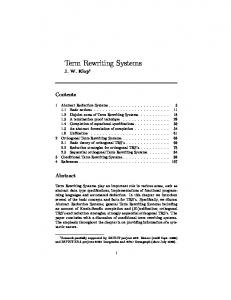
The tree rewriting model presented in this section is inspired by the Active XML (AXML) system developped at INRIA [4]. Active XML extends the framework of XML to describe semi-structured data by a dynamic component, describing data implicitly via service (function) calls. The evaluation of such calls is based on queries, resulting in extra data that can be added to the document tree. The abstract model is that of XML, i.e., unranked, unordered, labeled trees, together with a specification of the semantics for each service. Trees considered in this paper are labeled by tags from a finite set T . We will distinguish a subset Tvar ⊆ T of so-called tag variables. In addition, we use the special symbol $ to mark nodes where service calls insert new data. Trees are in the following unranked and unordered, with nodes labeled by T ∪ T$ , where T$ = T × {$}. We will not distinguish function/service nodes, since we consider here an abstract model for AXML documents, that is based on tree rewriting. We also do not consider multiple peers actually: their joint behavior can be described as the evolution of a unique document tree. A tree (V, parent, root, λ) consists of a set of nodes V with a distinguished node called root, a mapping parent : V \ {root} → V associating a node with its parent, and a mapping λ : V → T ∪ T$ labeling each node by a tag. Moreover, v1 [Play.com] v2 [MailOrder] v4 [Customer]
v3 [Catalog] v5 [Customer]
v8 [Cart]
v9 [Ordered]
v10 [Ordered]
v14 [skins]
v15 [LOTR]
v16 [skins]
v21 [£10]
v22 [£25]
v23 [£10]
v6 [Product]
v11 [Posted] v17 [day]
v18 [day]
v7 [Product]
v12 [Name]
v13 [Price]
v19 [skins]
v20 [£10]
Fig. 1. Tree document representing a catalog of products and customers history.
4 for each node v ∈ V , there is some k ≥ 0 such that parentk (v) = root. Such a tree is called a document if its labeling satisfies λ(V ) ⊆ T \ Tvar , that is, no node label uses a tag variable or the $ sign. A forest is a finite multiset of trees. Consider as an example the tree in Fig. 1. Informally, this tree represents a simplified version of the Play.com database, containing several products and information about customers. The subtrees of nodes v5 and v6 are not represented in the figure. The document shows two customers, one of which is currently shopping on the website with one product in her cart. This customer has 3 outstanding orders, one of which was posted 2 days ago (the counter days is encoded in unary in the tree). One can represents a tree in a term-like way. For example, to denote the empty catalog with no customer, we write v1 [Play.com](v2 [MailOrder], v3 [Catalog]), or if node names are irrelevant, [Play.com]([MailOrder], [Catalog]). Since trees are unordered, a tree can have several such representations. The atomic operations in our model are from a set R of guarded tree rewriting rules, as described below. On an abstract level we view a service s as described for instance by a regular expression R(s) over the set of rewriting rules R. For example, the following expression describes an order service on Play.com: (add-product + delete-product )∗ checkout. The tree resulting in the invocation of service s corresponds to the application of some sequence of rewriting rules in R(s). The atomic rewriting rules will use queries based on tree patterns (the descendant relation can be used together with the child relation), as described next. The symbol ⊎ used below stands for the disjoint union. Definition 1 (Tree-Pattern). A tree pattern (TP for short) is a tuple P = (V, parent, ancestor, root, λ), where (V, parent ⊎ ancestor, root, λ) is a tree. A tree pattern represents a set of trees that have a similar shape. As for trees, a TP can be described in a term-like way, ancestor-edges being represented by the symbol – (such edges are represented by a double line in the figures). For instance, the tree pattern LQBill shown in Fig. 2 can be written as w1 (–w2 (w3 (w4 ))), with λ(w1 ) = Play.com, λ(w2 ) = Ordered, λ(w3 ) = X, λ(w4 ) = Y (here X and Y are tag variables: X, Y ∈ Tvar ). This pattern represents trees with root “Play.com”, having a node “Ordered”, having itself a grandchild. Definition 2 (Matching). A tree T = (V, parent, λ, root) matches a TP P = (V ′ , parent′ , ancestor′ , λ′ , root′ ) if there exist two mappings f : V ′ → V and t : Tvar → T \ Tvar such that: – f (root′ ) = root, – For all v ∈ V ′ , λ(f (v)) = λ′ (v) if λ′ (v) ∈ / Tvar , and else λ(f (v)) = t(λ′ (v)), ′ – For all v ∈ V the following holds • If parent′ (v) is defined, then f (parent′ (v)) = parent(f (v)); • If ancestor′ (v) is defined, then f (ancestor′ (v)) is an ancestor of f (v) in T . Mappings (f, t) as above are called a matching between T and P . Furthermore, if f is injective, then (f, t) is called an injective matching.
5
f
v1 [play.com]
w1 [play.com]
node
node v2 [MailOrder]
v3 [Customer] v4 [Customer] v5 [Ordered]
T′
f
v6 [LOTR] v7 [£25]
w2 [Ordered]
LQBill
w3 [X]
f
w4 [Y]
f
Fig. 2. A tree T ′ matching the TP LQBill.
Fig. 2 shows an example of an injective matching between a tree T ′ and the TP LQBill. The only possible matching is f (w1 ) = v1 , f (w2 ) = v5 , f (w3 ) = v6 , f (w4 ) = v7 and t(X) =LOTR, t(Y ) = £25. With a matching f : V ′ → V we associate the mapping node : V \ f (V ′ ) → f (V ′ ) with node(v) being the lowest ancestor of v in f (V ′ ). For instance, for the mapping f matching T to P , node(v2 ) = node(v3 ) = node(v4 ) = v1 . Similarly to [2] we use in our model tree-pattern queries (TPQ for short, also called positive queries in [2]). Such queries have the form Q ; P , with Q a TP and P a tree, and the variables used in Q are also used in P . The TP Q selects tags in the tree. The result of a query = Q ; P on T is the forest query(T ) of all instantiations of P by matchings between T and Q. That is, for each matching (f, t) between T and Q we obtain an instance of P in which each Tvar -label X has been replaced by the tag t(X). For instance, let RQBill be the tree Product (Name(X),Price(Y)). Then the result of the TPQ (LQBill ; RQBill) on the tree in Fig. 1 is the forest depicted in Fig. 3. r1 [Product]
r6 [Product]
r2 [Name]
r3 [Price]
r7 [Name]
r8 [Price]
r4 [LOTR]
r5 [£25]
r9 [skins]
r10 [£10]
Fig. 3. Result forest of the TPQ LQBill ; RQBill on document T .
We now define a generic kind of (guarded) rewriting rules, as a model for active documents. Our rules are based on tree patterns, that occur in two distinct contexts. First, tree patterns are used for describing how the structure of the document tree changes through the rule - some subtrees might be deleted, new nodes can be added. Second, rules are guarded, and the guard condition is tested
6 via a TPQ. The role of the query is actually twofold: it is used in the pre-condition of the rule, and its result can enhance the information of the new tree. Definition 3 (TP rules). A TP rule is a tuple (left, query, guard, right), such that: – – – –
left is a TP (Vl , parentl , ancestorl , λl , rootl ) over T , right is a TP (Vr , parentr , ancestorr , λr , rootr ) over T ∪ T$ , query is a TPQ, guard is a set of forests.
We require the following additional properties: 1. all tag variables used in right appear also in left, and 2. ancestorr (x) = y iff x, y ∈ Vl ∩ Vr and ancestorl (x) = y. w1 (Play.com)
w1 (Play.com)
w5 (Customer)
w5 (Customer)
w2 (Ordered)
w6 (Processed) w7 (Bill,$)
left
right
Fig. 4. Tree patterns left and right of a rule. The additional conditions on right ensure that the right-hand side of a TP rule determines the form of the resulting tree, as it is explained below. For instance, Bill = (left, (LQBill ; RQBill), guard, right) is a TP rule, with left, right defined as in Fig. 4. Informally, the rule says that the system will process a Bill of the current order, and will tag the order as processed. The guard guard will be usually specified as a finite set of trees. In this case, the guard is fulfilled if the result of the query covers one of the tree of guard (see the decidable section 4). We first describe the semantics of a rule using the rule Bill as an example on the tree in Fig. 1. First, we compute an injective mapping f which maps the nodes w1 , w5 , w2 of left with the nodes v1 , v4 , v10 of T , respectively. We produce a new tree by rearranging and relabeling the nodes of T in the image of f , that is v1 , v4 , v10 . Some nodes can be deleted and others created. The resulting tree is shown in Fig. 5. We keep all nodes of T which are matched by nodes of left also present in right (v1 and v4 ), as well as their descendants by node−1 . That is, we keep all nodes labeled by vi in Fig. 5. In particular, a node matched in left which does not appear in right is deleted (as v10 , matched to w2 ), as well as its node−1 descendants (v16 and v23 ). The TP right makes it possible to create new nodes, present in right but not in left, as w6 , w7 . In addition, the TPQ query of the rule is used to attach a copy of the returned forest to all $-marked nodes of right. Furthermore, if the TPQ Q ; P uses in Q node name m common to
7 v1 [Play.com] v2 [MailOrder]
v3 [Catalog]
v4 [Customer]
v5 [Customer]
v8 [Cart]
v9 [Ordered]
w6 [Processed]
v14 [skins]
v15 [LOTR]
w7 [Bill]
v21 [£10]
v22 [£25]
v6 [Product]
v11 [Posted] v17 [day]
v18 [day]
v7 [Product]
v12 [Name]
v13 [Price]
v19 [skins]
v20 [£10]
r6 (Product)
r7 (Name)
r8 (Price)
r9 (skins)
r10 (£10) ′
Fig. 5. The tree document T resulting of the application of the rule Bill. left, then the results of the TPQ are restricted to those where m matches f (m). For instance, in the TP rule Bill, the TP LQBill uses names w1 , w2 common to left, hence the results of the TPQ (LQBill ; RQBill) are restricted to the particular order chosen by the matching f between T and left. The result is thus the subtree rooted at node r6 in Fig. 3, but not the subtree rooted at r1 , since it would require f (w2 ) = v9 , while f (w2 ) = v10 . This restriction is desirable, since we want to process a bill only for the products of this particular order. Here, w7 is $-marked, and the result forest is defined by nodes r6 , · · · r10 . More formally, let query = Q ; P be a TPQ and let (f, t) be an injective matching between T and left. Moreover, let Vl be the nodes of left and VQ those of Q. Let S1 , . . . , Sk be the trees composing the resulting forest query(T ), and let g1 , . . . , gk be the respective associated matchings (that is, gi : VQ → V and Si is the instantiation of P by gi ). Then we define queryf (T ) as the forest Si1 , . . . , Sil of those trees Sj such that gj agrees with f over Vl ∩ VQ . That is, queryf (T ) is the subset of query(T ) that is consistent with the matching f . We now turn to the formal semantics of rules. Definition 4 (Semantics of rules). Let T = (V, parent, λ, root) be a tree and R = (left, query = Q ; P, guard, right) be a rule, where left = (Vl , parentl , ancestorl , λl , rootl ) and right = (Vr , parentr , ancestorr , λr , rootr ). We say that R is enabled if there exists an injective matching (f, t) from left into T , such that queryf (T ) ∈ guard. The result of the application of R via (f, t) is the tree T ′ = (V ′ , parent′ , λ′ , root′ ) defined as follows: – V ′ = V1 ⊎ V2 ⊎ V3 ⊎ V4 with 1. V1 = f (Vl ∩ Vr ), % in the example on Fig. 5, V1 = {v1 , v4 } 2. V2 = node−1 (V1 ), % in the example on Fig. 5, V2 = {vi | i ∈ / {1, 4}} 3. V3 = f (Vr \ Vl ), % in the example on Fig. 5, V3 = {w6 , w7 } 4. V4 consists of distinct copies of the nodes of the forest queryf (T ), one for each node marked by $ in right. % in the example on Fig. 5, V4 = {ri | i ∈ {6, . . . , 10}} – Setting f (u) = u for all u ∈ V3 , we extend f : Vr ∪ Vl → V1 ⊎ V3 .
8 – root′ = f (rootr ). – Let u ∈ V1 and let u ¯ = f −1 (u) be the associated node in Vl ∩Vr . If λr (¯ u) ∈ / Tvar ′ then λ (u) = λr (¯ u), else λ′ (u) = t(λr (¯ u)). For all u 6= root′ , if parentr (¯ u) is defined, then parent′ (u) = f (parentr (¯ u)) else parent′ (u) = parent(u). – For all u ∈ V2 , parent′ (u) = parent(u) and λ′ (u) = λ(u). – For all u ∈ V3 \ {rootr }, parent′ (u) = f (parentr (u)) and λ′ (u) = λr (u). – To each node u ∈ V ′ marked by $, we add a copy of the forest queryf (T ) as children of u, and we unmark the node. Note that if x ∈ V2 , then its parent is in V1 ∪ V2 . The same stands if ancestorr (x) is defined. Note also that we indeed obtain a tree: for instance, if u ∈ V1 and parentr (¯ u) is not defined, then parent(u) is defined. This is because v = ancestorr (¯ u) is then defined, so by Def. 3, v = ancestorl (¯ u) in left, so that u = f (¯ u) cannot be the root of T . R
We write T → T ′ if T ′ can be obtained from T by applying the rule R. More generally, given a set of rules R we write T → T ′ if there is some rule R ∈ R with R ∗ T → T ′ , and T → T ′ for the reflexive-transitive closure of the previous relation. Notice that the tree T ′ matches right, through the matching f ′ : Vr → V ′ defined by f ′ (v) = f (v) if v ∈ Vr ∩ Vl , and f ′ (v) = v if v ∈ Vr \ Vl . Example (Play.com rules). To show how easily rules can be defined, we describe now some rules of the Play.com system. When the rule does not use a query or a guard, we only describe the left and right components. – The rule New-Customer adds a new customer and its cart. • left = w1 [Play.com](w2 [MailOrder]) • right =w1 [Play.com](w2 [MailOrder](w3 [Customer](w4 [Cart]))). – Every new day, if a posted parcel has not yet been received yet, then the day counter is incremented. • left = w1 [Play.com](–w2 [Posted]) • right = w1 [Play.com](–w2 [Posted](w3 [day])) – If after 21 days a posted parcel is still not received, the customer can require a payback. We use the guard to ensure this time limit. Notice that the query is Q ; P , where Q uses the same w2 as in left, that is the number of days will be counted only for this particular parcel. • left = w1 [Play.com](–w2 [Posted]) • Q= w1 [Play.com](–w2 [Posted](w3 [day]) • P = x4 [day] • guard: a forest containing at least 21 trees (and possibly more nodes) whose root is labeled day. • right = w1 [Play.com].
3
Static Analysis of TPRS
We assume from now on that an active document is given by a tree pattern rewriting systems (TPRS) (T, R), consisting of a set R of TP rules and a T labeled tree T . That is, we assume that each service corresponds to a rule. Our
9 results are easily seen to hold in the more general setting where services are regular expressions over R. A tree T with node set V is subsumed by a tree T ′ with node set V ′ , noted T � T ′ , if there is an injective mapping from V to V ′ that preserves the labeling, the root, and the parent relation. A forest F is subsumed by a forest F ′ , written F � F ′ , if F is mapped injectively into F ′ such that each tree in F is subsumed by its image in F ′ . Similarly, a TP P with node set V is subsumed by a TP P ′ with node set V ′ , if there is an injective mapping from V to V ′ that preserves the labeling, the root, the parent and the ancestor relations. With a TPRS (T, R) we can associate the (infinite-state) transition system ∗ hS(T, R), →i with S(T, R) = {T ′ | T → T ′ }. We are interested in checking the following properties: – – – –
Termination: Are all derivation chains T → T1 → T2 → · · · of (T, R) finite? Finite-state property: Is the set S(T, R) of reachable trees finite? Reachability: Given (T, R) and a tree T ′ , is T ′ reachable in (T, R)? Confluence (joinability): For any pair of trees T1 , T2 ∈ S(T, R), does there ∗ ∗ exist some T ′ such that T1 → T ′ and T2 → T ′ ? – Pattern reachability (coverability): Given (T, R) and a tree pattern P , does ∗ T → T ′ hold for some T ′ matching P ? – Weak confluence: From any pair of trees T1 , T2 ∈ S(T, R), does there exist ∗ ∗ T1′ � T2′ such that T1 → T1′ and T2 → T2′ ? For instance, pattern reachability is a key property when we want to talk about the reachability of some pattern. For example, we might ask whether an already cancelled order could still be delivered, which would mean a problem in the system. For this, it suffices to tag cancelled orders with a special symbol #, and check for the pattern w1 [Play.com](–w2 [delivered](w3 [#])). This is the same kind of properties which are checked in [3]. As expected, any of the non-trivial questions above is undecidable in the general case, see Theorem 1 below. We are thus looking for relevant restrictions yielding decidability of at least some of these problems. In the next section we consider a subclass of TPRS, which is a special instance of the so-called well-structured systems. We say that (T, R) is positive if all guards occurring in the rules from R, are upward-closed. This means that for every guard G, and all forests F, F ′ with F � F ′ , F ∈ G implies F ′ ∈ G, too. In particular, if a rule R in a positive system is enabled for a tree T , then R is enabled for any tree T ′ that subsumes T . The reason is that for any TPQ query, we have that for every tree T1′ in query(T ′ ), there is some tree T1 in query(T ) such that T1 is subsumed by T1′ . Notice that positive TPRS allow deletion of nodes, so they are more powerful than the positive AXML systems considered in [2]. The next theorem shows that upward-closed guards alone do not suffice for obtaining decidability of termination: Theorem 1. Any two-counter machine M can be simulated by a positive TPRS (T, R) in such a way that M terminates iff (T, R) terminates.
10 Theorem 1 shows that any non trivial property is undecidable for positive TPRS without further restrictions. However, notice that the proof of the above result needs trees of unbounded depth. A realistic restriction in the XML setting is to consider only trees of bounded depth: XML documents are usually large, but shallow. A TPRS (T, R) is called depth-bounded, if there exists some fixed ∗ integer K such that every tree T ′ with T → T ′ has depth at most K. Of course, Theorem 1 implies that it is undecidable to know whether a TPRS is depthbounded. However, in many real-life examples this property is easily seen to hold (see e.g. the Play.com example, which has depth at most 8).
4
Decidability for positive and depth-bounded TPRS
For positive and depth-bounded TPRS, we can apply well-known techniques from the verification of infinite-state systems that are well-structured. Wellstructured transition systems were considered independently by [1,8] and they cover many interesting models, such as Petri nets or lossy channel systems. We recall first some basics of well-structured systems. Definition 5. A well-quasi-order (wqo) on a set X is a preorder � such that in every infinite sequence (xn )n≥0 ⊆ X, there exist some indices i < j with xi � xj . In general, the “subsumed” relation � on the set X of T -labeled trees is not a wqo.1 However, using Higman’s lemma (see, e.g., [6, Chap. 12]), one can show that � is a wqo on the set of trees of depth at most K (for any fixed K): Proposition 1. Fix K ∈ N, and let XK denote the set of unordered T -labeled trees of depth at most K. The “subsumed” relation � ⊆ XK × XK is a wqo. By the previous statement, a positive and depth-bounded TPRS (T, R) yields a well-structured transition system hS(T, R), →i as defined in [8] (see also2 [1]). This follows from the transition relation → being upward compatible: whenever R R T → T ′ and T � T1 , there exists T1′ with T1 → T1′ and T ′ � T1′ . For the next theorem we need first some notation. Given a set X and a preorder �, we denote by ↑X the upward closure {T ′ | T � T ′ for some T ∈ X} of X. By min(X) we denote the set of minimal elements3 of X. Finally, by Pred(X) we denote the set of immediate predecessors of elements of X. Note that whenever the transition relation → is upward compatible and X upwardclosed, the set Pred(X) is upward-closed, too. 1
2
3
Indeed consider the sequence of trees (Tn )n≥0 where for each n ≥ 0, Tn is the tree formed by a single branch of length n + 1 whose internal nodes are labeled by a and the unique leaf is labeled by b. As shown in the proof of Thm. 2, hS(T, R), →i is also well-structured as defined in [1], which requires in addition that the set of predecessors of upward-closed sets is effectively computable. For a wqo (X, �) and Y ⊆ X, the set min(Y )/∼ is finite, where ∼ = � ∩ �−1 . For the subsumed relation �, note that ∼ is the identity.
11 Since the subsumed relation � is a wqo, the � relation on forests is a wqo as well. Thus, each guard G in a positive, depth-bounded TPRS (T, R) can be described by the (finite) set of forests min(G). The size |G| of G is the maximal size of a forest in min(G). Theorem 2. Termination and pattern reachability are both decidable for positive and depth-bounded TPRS. Proof. First, termination is decidable for well-structured systems such that 1) � is decidable, 2) → is computable and 3) upward compatible, see [8, Thm. 4.6]. For pattern reachability, it is easy to see that the set of trees of depth bounded by some K which matches a TP P is upward-closed, and that the set of its minimal elements is effectively computable. We can thus use [1], which shows decidability of the reachability of ↑T under the assumption that the set min(Pred(↑T )) is computable. This allows to use the obvious backward exploration algorithm. From now on, we fix the tree T and the bound K of the system (T0 , R). Let us also fix a rule R = (left, query, guard, right). It suffices to consider the finite set SR (T ) of all trees T ′ of size at most R
|T | + |left| + K|query||guard| with T ′ −→ T . Then, defining M as the set of S minimal elements of R∈R SR (T ), we get by definition M ⊆ min(Pred(↑T )). Let us now show that M = min(Pred(↑T )). Let T1 ∈ min(Pred(↑T )). Thus, R there exist some rule R and some injective matching (f, t) with T1 −→ T via ′ ′ (f, t). Let also F ∈ min(guard) be a forest with F � F , where F is the result of query on T1 (compatible with the matching f ). The nodes of T1 can be partitioned into 4 sets V1 , V2 , V3′ , V2′ (below Vl are the nodes of left and Vr those of right): V1 = f (Vl ∩ Vr ), V2 = node−1 (V1 ), V3′ = f (Vl \ Vr ), V2′ = node−1 (V3′ ). Notice that V1 and V2 are common with T (see Def. 4), hence |T1 | ≤ |T | + |V3′ | + |V2′ |. Now, |V3′ | ≤ |left|. We now explain that V2′ has at most |query||guard| leaves, hence |V2′ | ≤ K|query||guard| which shows that T1 ∈ SR (T ). Otherwise one can delete a leaf from V2′ and get a tree R T1′ � T1 with T1′ −→ T (via (f, t)), and still F � F ′′ , where F ′′ denotes the result of query on T1′ . This contradicts the minimality of T1 . 2 On the negative side, depth-bounded well-structured systems can simulate reset Petri nets (i.e., nets with an additional transition that empties a place), hence we can deduce the following from known results: Theorem 3. Exact reachability, confluence, weak confluence and the finite-state property are undecidable for positive and depth-bounded TPRS. On the positive side, we can show that the finite-state property is decidable for positive, depth-bounded TPRS, that are strict, i.e., such that for any rule (left, query, guard, right), we require Vleft ⊆ Vright . One cannot encode reset Petri nets with such systems because deletion is no longer possible (actually one can only relabel an existing node and create new nodes). Strict systems enjoy the R additional property that whenever T → T ′ and T ≺ T1 , there exists T1′ with R T1 → T1′ and T ′ ≺ T1′ (notice that for non strict systems, we can only guarantee that T ′ � T1′ ). The results from [8] yield the following theorem.
12 Theorem 4. The finite-state property and reachability are decidable for TPRS that are positive, depth-bounded, and strict. Note that the finite-state property is not very interesting in itself, but if it holds, then the other problems become decidable as we are dealing with a finitestate system. In particular, in order to test for confluence, it suffices to test that (S(T, R), →) has a unique maximal strongly connected component. Note that reachability is decidable for positive, depth-bounded and strict TPRS simply because T → T ′ implies that |T | ≤ |T ′ |, and then it suffices to look for reachability of a tree T1 in the finite state system {T ′ | |T ′ | ≤ |T1 |}. The table below sums up the results we obtained so far. It presents (un)decidability results concerning the various classes of positive TPRS we considered (depthbounded and strict). The negative results about strict TPRS come from Theorem 1 (results on strict TPRS are obtained using slight variations of our proofs). Term., FS, Reach., P-reach, Confl. and W-confl. stand respectively for termination, finite state property, reachability, pattern reachability, confluence and weak confluence. Model Strict Depth-Bounded Depth-Bounded & Strict
5
Term. FS Reach. P-reach. Confl. W-confl. U D D
U U D
U U D
U D D
U U U
U U U
Lower bounds and extensions
Decidability results are obtained with non-constructive proofs coming from Higman’s Lemma. This ensures termination of the algorithms, but without yielding complexity bounds. It is thus relevant to obtain lower bounds for these results. Theorem 5. The following problems have at least non-elementary complexity: – Input: A TP P , a TPRS system (S, R) and an integer k such that the depth of (S, R) is bounded by k. – Problem1: Is the pattern P reachable in (S, R)? – Problem2: Does (S, R) terminate, equiv., does it have an infinite path? Proof. Let tower(0, n) = n and tower(k + 1, n) = 2tower(k,n) . Let M be an n 7→ tower(k, n)-space bounded deterministic Turing machine and x be an input of M . Denote by log∗ n the smallest integer m such that n ≤ tower(m, 2) and let K = k + log∗ |x|, so that the computation of M on x uses at most tower(k, |x|) ≤ tower(K, 2) tape cells. We build a (K + 1)-depth bounded TPRS of size O(|M | + |x|) simulating M on x. Informally, we encode each configuration of M by a tree. Each cell is encoded by a subtree of the root, labeled at its own root by the cell content, with the forest
13 below it encoding the position of the cell. Since such a position is smaller than tower(K, 2), it can itself be encoded recursively by a forest of depth at most K (such a recursive encoding of large integers, by words, has already been used in [15]). For instance, one can encode integers from 0 to 15 = tower(2, 2) − 1 at depth 2. The forest of Fig. 6 encodes 13 (1101 in binary). To recover its position, each bit of the base 2 representation has under itself a forest of depth 1 encoding its position (recursively with the same encoding scheme). For instance, the leftmost 1 is at position 00, which is encoded by the forest {[0]([0]), [0]([1])}. Let N = tower(K, 2) − 1. We encode the configuration C of M with tape content a0 · · · aN , current state q and scanned position m, by the forest FC = a ¯0 (F0K ) · · · a ¯N (FNK ) of depth K + 1, with a ¯m = [am , q] and a ¯i = [ai ] for i 6= m, K where Fi is the forest of depth K encoding the number i ≤ N . The head position is thus doubly tagged: by the letter, and by the state. Such a node with a double tag [α, β] is said marked by β, or a β-node. In order to navigate through the cells, we use for each level ℓ ≤ K an additional placeholder node, child of the root, named cℓ for holding a level ℓ counter below it. The idea is that the counter attached below cK will be able to count up to N , and hence can pinpoint a tape position. The other counters are needed in the inductive process. During the computation, additional markers will be used either as pebbles, or to guide the control. Figure 7 shows a typical tree reached during the computation. The rules of the TPRS are set up so that it performs successively the following actions: 1. It creates the forest FC0 , and attaches it under the root, leaving cK labeled by [cK , run] and for ℓ < K, cℓ labeled by [cℓ , end]. 2. It simulates repeatedly transitions of M , stopping if the final state is reached. We only show how to encode transitions. The generation of the initial configuration, starting from the tree [M ]([c0 , end], . . . , [cK−1 , end], [cK , create-init-config]), is done using similar routines. We use a finite set of rules without query/guard part. Although the TPRS will be nondeterministic, appropriate tags shall ensure that rules applicable at some step have all the same left member. When the TPRS discovers that a nondeterministic guess was wrong, it blocks. Therefore, if M halts on x, then the TPRS always terminate. If M does not halt on x, then the corresponding run of the TPRS where all guesses are correct does not either. This ensures termination iff M halts on x. To simulate a transition, the TPRS first performs the changes in the configuration, nondeterministically guessing the new head position. To check whether the head has been properly placed, it ∗-marks the original head position. The node cK marked by { run, check-suc1, check-suc2, . . . , check-pred1,check-pred2. . . } [1]
[1]
[0]
[1]
[0]
[0]
[0]
[1]
[1]
[0]
[1]
[1]
[0]
[1]
[0]
[1]
[0]
[1]
[0]
[1]
Fig. 6. A level 2 counter encoding 13.
14 [M ] [b]
[b, ∗]
[b, q]
[a]
[c0 ,true] [c1 ,cmp-compare-bits] [c2 ,check-suc3]
[0]
[0]
[0]
[1]
[1]
[0, ∗1 ]
[1]
[1]
[0]
[1]
[0]
[1]
[0]
[1]
[0]
[1]
[1]
[1]
[0, ∗′1 ]
[0]
[1]
Fig. 7. The tree coding the tape b b q b a of the Turing machine M .
(for instance, check-suc needs several steps) encodes the current stage of the sima/b/→
ulation. For instance, to simulate a transition p −−−−→ q, we use the rule: − left = r[M ](x[a, p], y[X], z[cK , run]), − right = r[M ](x[b, ∗], y[X, q], z[cK , check-suc1]), slightly abusing notation: we use a double tag involving a variable, to abbreviate a finite set of rules (with the obvious interpretation). To complete the simulation of the transition, the TPRS checks whether the position written below the node pinpointed by q is a successor of that below the node pinpointed by ∗. If yes, it deletes the mark ∗, and labels cK back to [cK , run]. If not, the head position was incorrectly guessed and the system blocks. The steps of check-suc, which checks that the nodes marked by ∗ and q occur successively, are first a copy under cK of the level K counter located below the ∗-node, then an increment of that copy, and a comparison of the result to the counter below the q-node. We use auxiliary markers ∗ℓ , ∗′ℓ for each level ℓ, attached to nodes below an ℓ counter: ∗ℓ in the part of the tree representing the configuration, and ∗′ℓ under some ci , i > ℓ. We define inductively rules to achieve the following tasks for each level ℓ ≤ K: – – – – –
copy(ℓ) copies below the ∗′ℓ -marked node the level ℓ counters found below cℓ . increment(ℓ) increments the level ℓ counter below cℓ . compare(ℓ) compares level ℓ counters below cℓ and below the ∗ℓ -marked node. test-max(ℓ) tests if the level ℓ counter below cℓ has its maximal value. zero(ℓ) generates under cℓ the level ℓ counter F0ℓ .
Each task of level ℓ is implemented by a sequence of tasks of level (ℓ − 1), using some fresh tags to correctly organize the order of these level (ℓ − 1) tasks. See [9] for some detailed rules. 2 The bounded depth restriction needed for our decidability results can be relaxed if we forbid the use of the direct parent-child edges in tree patterns. This leads to the following preorder on unranked, unordered T -labeled trees, which is a well quasi-order by Kruskal’s theorem (see [6, Chap. 12]). For two trees T, T ′ with sets of nodes V, V ′ respectively, we write T ⋖ T ′ , if there is an injective mapping from V to V ′ that preserves the labeling, the root, and the ancestor relation. So compared to the relation � used previously, we do not require that the parent relation is preserved.
15 Clearly, we need to restrict the TPRS rules in order to obtain well-structured systems. Namely we require that all TP occurring in query and left use only ancestor edges (right can still use parent edges, but the parent relation cannot be tested for). We call such TPRS undirected. Using similar proofs as in Sect. 4, we get the same decidability results. For the lower bound we obtain a stronger result, by encoding reachability for lossy channel systems (LCS). These are finite-state machines communicating over FIFO channels that can loose arbitrary many messages. Reachability for LCS has non primitive recursive complexity [14], already for LCSs made up of two finite-state machines and two channels [5]. Theorem 6. Termination and pattern reachability have at least non primitive recursive complexity for undirected TPRS.
References 1. P. A. Abdulla, K. Cerans, B. Jonsson, and Y.-K. Tsay. General decidability theorems for infinite-state systems. In LICS’96, pp. 313–321. IEEE Comp. Soc., 1996. 2. S. Abiteboul, O. Benjelloun, and T. Milo. Positive Active XML. In PODS’04, pp. 35–45. ACM, 2004. 3. S. Abiteboul, L. Segoufin, and V. Vianu. Static Analysis of Active XML Services. In PODS’08. ACM, 2008. To appear. 4. Active XML. http://www.activexml.net/. 5. P. Chambart and Ph. Schnoebelen. The Ordinal Recursive Complexity of Lossy Channel Systems. In LICS’08. IEEE Comp. Soc., 2008. To appear. 6. R. Diestel. Graph theory. 2005. http://www.math.uni-hamburg.de/home/diestel. 7. C. Dufourd, A. Finkel and Ph. Schnoebelen. Reset Nets between Decidability and Undecidability. In ICALP’98, LNCS 1443, pp. 103–115. Springer, 1998. 8. A. Finkel and Ph. Schnoebelen. Well-structured transition systems everywhere! Theor. Comput. Sci., 256(1-2):63–92, 2001. 9. B. Genest, A. Muscholl, O. Serre, M. Zeitoun. Tree Pattern Rewrite Systems. Internal report available at http://www.crans.org/∼ genest/GMSZ08.pdf. 10. N. Dershowitz and D. Plaisted. Chapter 9 in: Handbook of Automated Reasoning, vol. 1, A. Robinson and A. Voronkov eds, Elsevier (2001). 11. L. Libkin. Logics over unranked trees: an overview. Logical Methods in Computer Science, 2(3), 2006. 12. Ch. L¨ oding and A. Spelten. Transition Graphs of Rewriting Systems over Unranked Trees. In MFCS’07, LNCS 4708, pp. 67-77. Springer, 2007. 13. F. Neven. Automata, Logic, and XML. In CSL’02, LNCS 2471, pp. 2–26. Springer, 2002. 14. Ph. Schnoebelen. Verifying Lossy Channel Systems has Nonprimitive Recursive Complexity. Inf. Process. Lett. 83(5):251–261, 2002. 15. I. Walukiewicz. Difficult Configurations—on the Complexity of LTrL. Form. Methods Syst. Des., 26(1): 27–43. Kluwer, 2005. Short version in ICALP’98, LNCS 1443.