Tree-Structured Linear-Phase Nyquist FIR Filter Interpolators and Decimators Håkan Johansson, Amir Eghbali, and Jimmie Lahti Division of Electronics Systems, Department of Electrical Engineering, Linköping University, Sweden Email:
[email protected],
[email protected],
[email protected]
Abstract— This paper introduces a new class of linear-phase Nyquist (𝑀 th-band) FIR interpolators and decimators based on tree structures. Through design examples, it is shown that the proposed converter structures have a substantially lower computational complexity than the conventional single-stage converter structures. The complexity is comparable to that of multi-stage Nyquist converters, although the proposed ones tend to have a somewhat higher complexity. A main advantage of the proposed structures is however that they can be used for arbitrary integer conversion factors, thus including prime numbers which cannot be handled by the regular multi-stage Nyquist converters.
II. S TRUCTURES FOR O DD I NTERPOLATION FACTORS The proposed interpolator structures are most easily described in terms of non-causal filters. The corresponding causal structures are readily obtained by introducing delay elements appropriately. Further, for an odd interpolation factor 𝑀 , it is here appropriate to assume that the overall transfer function, 𝐻(𝑧), can be expressed in polyphase form as (𝑀 −1)/2
Interpolation and decimation filters are important signal processing blocks as conversions between different sampling frequencies are required in many different applications [1]. During the past decades, several different interpolator and decimator structures have been introduced in different applications, aiming at reducing the computational complexity of the conversions. Many recent papers address reconfigurable converters [2]–[5] which are required in, for example, emerging communication systems so as to support different standards and operation modes [6]–[8]. However, as will be demonstrated in this paper, there is still room for further improvements also for fixed converters which may also serve as efficient parts of reconfigurable converters. To this end, this paper introduces a new class of linearphase Nyquist (also called 𝑀 th-band) FIR interpolator and decimator structures. Nyquist filters find applications in several contexts, like filter banks, spectrum sensing, and pulse shaping [9]–[12]. In the rest of this paper, only the interpolation will be discussed as a decimator structure can be readily derived by transposing the corresponding interpolator structure. In the proposed class of interpolators, the overall interpolation is achieved through a tree structure whose branches, from the root node to the leaf nodes, realize the different polyphase components required. Compared to conventional single-stage interpolators, the proposed ones have a substantially lower computational complexity. It is comparable to that of multi-stage Nyquist interpolators [13], although the proposed ones tend to have a somewhat higher complexity. However, the drawback of the regular multi-stage Nyquist interpolators is that they cannot be used for conversions by prime numbers. The proposed interpolators, on the other hand, can be used for arbitrary integer conversion factors. An additional advantage of the proposed interpolators is that all filtering operations occur at the input sampling rate, like in regular single-stage interpolators. In the multi-stage Nyquist interpolators, the filters in one or several stages operate at a higher rate than the input rate. It is possible to parallellize the multi-stage structures so that all filtering operations take place at the input rate but the derivation and schemes may become rather involved when the number of stages increases. Following this introduction, Sections II and III introduce the proposed interpolator structures for odd and even conversion factors, respectively. Section IV describes the design whereas Section V provides design examples. Finally, Section VI concludes the paper.
978-1-4673-0219-7/12/$31.00 ©2012 IEEE
∑
𝐻(𝑧) =
I. I NTRODUCTION
2329
𝑧 −𝑚 𝐻𝑚 (𝑧 𝑀 ).
(1)
𝑚=−(𝑀 −1)/2
The proposed tree structures are then derived utilizing the following two facts. Fact 1: For a non-causal 𝑀 th-band filter with a transfer function according to (1), the frequency responses of 𝑧 −𝑚 𝐻𝑚 (𝑧 𝑀 ) must approximately satisfy [14] 𝑒−𝑗𝜔𝑇 𝑚 𝐻𝑚 (𝑒𝑗𝜔𝑇 𝑀 ) = 1, 𝜔𝑇 ∈ [0, (1 − 𝜌)𝜋/𝑀 ], 0 < 𝜌 < 1, (2) assuming that the passband gain is 𝑀 to preserve the energy in the interpolation process. From this equation, it follows that the frequency response of the polyphase components 𝐻𝑚 (𝑧) must approximately satisfy 𝐻𝑚 (𝑒𝑗𝜔𝑇 ) = 𝑒𝑗𝜔𝑇 𝑚/𝑀 , 𝜔𝑇 ∈ [0, (1 − 𝜌)𝜋].
(3)
That is, the polyphase components should approximate fractionaldelay (FD) filters with delays of 𝑚/𝑀, 𝑚 = −(𝑀 − 1)/2, −(𝑀 − 1)/2 + 1, . . . , (𝑀 − 1)/2. It is also noted that, for 𝑚 = 0, we have the trivial polyphase component 𝐻0 (𝑒𝑗𝜔𝑇 ) = 1. Fact 2: The sum of two allpass functions 𝑒−𝑗𝜔𝑇 𝑑1 and 𝑒−𝑗𝜔𝑇 𝑑2 can be written as 𝑒
−𝑗𝜔𝑇 𝑑1
+𝑒
−𝑗𝜔𝑇 𝑑2
=𝑒
−𝑗𝜔𝑇 (𝑑1 +𝑑2 )/2
(
(𝑑1 − 𝑑2 )𝜔𝑇 × 2 cos 2
) .
(4) This means that, if we have realized two FD filters with the delays 𝑑1 and 𝑑2 , respectively, we can generate a new FD filter with a delay of (𝑑1 + 𝑑2 )/2 by first summing the outputs of the two filters and then applying the so obtained result to a linear-phase filter that equalizes the term 2 cos ((𝑑1 − 𝑑2 )𝜔𝑇 /2). From the above two facts, an add-equalize principle follows which can be used to generate all of the polyphase components of an 𝑀 thband filter. To this end, we introduce the quantity 𝑃 given as 𝑃 = 2𝑅−1 ,
(5)
𝑅 = ⌈log2 (𝑀 − 1)⌉ .
(6)
where
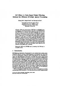
Polyphase branches realizing fractional delays m/M, m = -4,...4.
G3(z)
G3(z) In
3/M
1/M
G2(z)
G12(z)
, 𝑟 = 2, 3, . . . , 𝑅.
(7)
Therefore, these two filters can be efficiently realized as the sum and difference of two linear-phase filters 𝐶1 (𝑧) and 𝐶2 (𝑧) given by
-1/M
𝐶1 (𝑧) =
-2/M G3(z)
)
𝐺12 (𝑧) = 𝐺11 (𝑧 −1 ) ⇔ 𝑔12 (𝑛) = 𝑔11 (−𝑛).
0 G3(z)
𝜔𝑇 ×2𝑅−𝑟 𝑀
, 𝑅,)are used for equalizing As the subfilters 𝐺𝑟 (𝑧), 𝑟 = 2, ( 3, . . .𝑅−𝑟 the real-valued functions 2 cos 𝜔𝑇 ×2 , they are selected to 𝑀 be Type-I linear-phase FIR filters, thus of even order and with symmetric impulse responses [15]. Further, since 𝐺11 (𝑧) and 𝐺12 (𝑧) are to realize 𝑒−𝑗𝜔𝑇 𝑃/𝑀 and 𝑒𝑗𝜔𝑇 𝑃/𝑀 , and because 𝑒𝑗𝜔𝑇 𝑃/𝑀 is the conjugate of 𝑒−𝑗𝜔𝑇 𝑃/𝑀 , 𝐺12 (𝑧) is here determined by 𝐺11 (𝑧) as
2/M
G2(z)
(
A. Linear-Phase Filters
4/M
G11(z)
Fig. 1.
2, 4, 8, . . . , 𝑃, or, equivalently, 2 cos
𝐺11 (𝑧) + 𝐺12 (𝑧) 2
(8)
and 𝐺11 (𝑧) − 𝐺12 (𝑧) . (9) 2 The filter 𝐶1 (𝑧) is then a symmetric linear-phase filter (Type I) whereas 𝐶2 (𝑧) is an anti-symmetric linear-phase filter (Type III). The filters 𝐺11 (𝑧) and 𝐺12 (𝑧) are then realized as 𝐶2 (𝑧) =
-3/M -4/M
Tree structure used for interpolation by 𝑀 ∈ [6, 7, 8, 9].
This means that 𝑅 = 2 for 𝑀 = 5, 𝑅 = 3 for 𝑀 ∈ [7, 9], 𝑅 = 4 for 𝑀 ∈ [11, 13, 15, 17], etc. Note also that 𝑀 = 3 is a feasible case, with 𝑅 = 1, but this coincides with a regular three-band filter. The first step is now to realize the two FD filters 𝑒−𝑗𝜔𝑇 𝑃/𝑀 and 𝑒𝑗𝜔𝑇 𝑃/𝑀 . Then, we pair-wise add their outputs to( the trivial ) 𝑃 and gives 𝑒−𝑗𝜔𝑇 𝑃/(2𝑀 ) × 2 cos 𝜔𝑇 filter 𝐻0 (𝑒𝑗𝜔𝑇 ) = 1( which 2𝑀 ) ) 𝜔𝑇 𝑃 , respectively. By equalizing the two terms ×2 cos 𝑒𝑗𝜔𝑇 𝑃/(2𝑀 2𝑀 ( 𝑃) , we have then realized the two FD filters 𝑒−𝑗𝜔𝑇 𝑃/(2𝑀 ) 2 cos 𝜔𝑇 2𝑀 and 𝑒𝑗𝜔𝑇 𝑃/(2𝑀 ) . Consequently, we have now five FD filters in total, viz. 𝑒−𝑗𝜔𝑇 𝑃/𝑀 , 𝑒−𝑗𝜔𝑇 𝑃/(2𝑀 ) , 1, 𝑒𝑗𝜔𝑇 𝑃/(2𝑀 ) , and 𝑒𝑗𝜔𝑇 𝑃/𝑀 . The next step is to generate four new FD filters by pair-wise adding the outputs (of two) adjacent FD filters and then equalizing the four 𝑃 . This gives a total of nine FD filters with delays terms 2 cos 𝜔𝑇 4𝑀 equally spaced between −𝑃/𝑀 and 𝑃/𝑀 . Continuing in the same manner, we have after 𝑅 steps generated 2𝑃 +1 FD filters with delays equally spaced between −𝑃/𝑀 and 𝑃/𝑀 . Finally, 𝑀 of these FD filters, for 𝑚 = −(𝑀 − 1)/2, −(𝑀 − 1)/2 + 1, . . . , (𝑀 − 1)/2, are used to realize the polyphase components 𝐻𝑚 (𝑧) in (1). Figure 1 shows the tree structure for 𝑅 = 3 and 𝑃 = 2 which is used for 𝑀 = 7 and 𝑀 = 9, and also for the even numbers (to be discussed below) 𝑀 = 6 and 𝑀 = 8. When 𝑀 = 6 or 𝑀 = 7, only the branches for 𝑚 = −3, −2, . . . , 3 are used whereas all branches are used for 𝑀 = 8 and 𝑀 = 9. Not using the branches for 𝑚 = −4 and 𝑚 = 4 does not offer any savings in this structure as all subfilters are needed for generation of the remaining outputs. In the general structure, with 𝑅 levels, some of the subfilters in the last level(s) can be eliminated, depending on how many branches that are not used in (1). Further, the subfilters 𝐺11 (𝑧) and 𝐺12 (𝑧) in Fig. 1 are used for realizing the FD filters 𝑒−𝑗𝜔𝑇 𝑃/𝑀 and 𝑒𝑗𝜔𝑇 𝑃/𝑀 , respectively, ( 𝜔𝑇 𝑃 ) whereas ( 𝜔𝑇𝐺𝑃2)(𝑧) and 𝐺3 (𝑧) are used for equalizing 2 cos 2𝑀 and 2 cos 4𝑀 , respectively. In the general structure, with 𝑅 levels, 𝐺11 (𝑧) and 𝐺12 (𝑧) still realize 𝑒−𝑗𝜔𝑇 𝑃/𝑀 and 𝑒𝑗𝜔𝑇(𝑃/𝑀 , )respec𝑃 tively, whereas 𝐺𝑟 (𝑧), 𝑟 = 2, 3, . . . , 𝑅, equalize 2 cos 𝜔𝑇 ,𝑝= 𝑝𝑀
2330
𝐺11 (𝑧) = 𝐶1 (𝑧) + 𝐶2 (𝑧)
(10)
𝐺12 (𝑧) = 𝐶1 (𝑧) − 𝐶2 (𝑧).
(11)
and
In this way, the multiplication complexity of the two unsymmetric filters 𝐺11 (𝑧) and 𝐺12 (𝑧) is reduced by a factor of two as compared to their separate realizations. Furthermore, as the proposed overall structure then consists of linear-phase subfilters only, and as each polyphase component in (1) contains also its complex conjugate due to (3), a linear-phase overall filter 𝐻(𝑧) is obtained. III. S TRUCTURES FOR E VEN I NTERPOLATION FACTORS The structures for even interpolation factors are derived in essentially the same way. Some minor modifications are however required as described in this section. Firstly, the overall transfer function is here expressed in the polyphase form 𝑀/2
𝐻(𝑧) =
∑
𝑤 × 𝑧 −𝑚 𝐻𝑚 (𝑧 𝑀 ).
(12)
𝑚=−𝑀/2
where { 𝑤=
1, 𝑚 = −𝑀/2 + 1, −𝑀/2 + 2, . . . , 𝑀/2 − 1 1/2, ∣𝑚∣ = 𝑀/2.
(13)
The polyphase representation in (12) contains 𝑀 + 1 components instead of the conventional decomposition with 𝑀 terms. The reason is that, in this way, a linear-phase overall 𝐻(𝑧) filter is again obtained as each polyphase component in (12) then contains also its complex conjugate due to (3). Secondly, 𝑅 is now given by 𝑅 = ⌈log2 (𝑀 )⌉ ,
(14)
which means that 𝑅 = 2 for 𝑀 = 4, 𝑅 = 3 for 𝑀 ∈ [6, 8], 𝑅 = 4 for 𝑀 ∈ [10, 12, 14, 16], etc.
IV. F ILTER D ESIGN In this paper, minimax design [16] is considered but other types of design criteria, like least-squares [17], can be used as well after some minor appropriate modifications. We minimize the maximum of the modulus of the error function 𝐸(𝑗𝜔𝑇 ) given by 𝐸(𝑗𝜔𝑇 ) = 𝐻(𝑒𝑗𝜔𝑇 ) − 𝐷(𝑗𝜔𝑇 ),
𝜔𝑇 ∈ Ω
(15)
where 𝐷(𝑗𝜔𝑇 ) is the desired function to be approximated. As the overall filters are 𝑀 th-band filters, it normally suffices to consider the stopband in the filter design. This is because the passband and stopband ripples of an 𝑀 th band FIR filter, say 𝛿𝑐 and 𝛿𝑠 , are related as 𝛿𝑐 ≤ (𝑀 −1)𝛿𝑠 [15]. Consequently, Ω is here the stopband region where the desired function 𝐷(𝑗𝜔𝑇 ) is zero. Two different stopband region cases are considered: Ω = [(1 + 𝜌)𝜋/𝑀, 𝜋] [ ( )] ∪ (2𝑝−1+𝜌)𝜋 , min (2𝑝+1−𝜌)𝜋 ,𝜋 . Ω = ⌊𝑀/2⌋ 𝑝=1 𝑀 𝑀 (16) Here, Case 1 covers the whole band from the stopband edge (1 + 𝜌)𝜋/𝑀 up to 𝜋, whereas Case 2 includes don’t-care bands centered on (2𝑝 + 1)𝜋/𝑀, 𝑝 = 1, 2, . . . , ⌊(𝑀 − 1)/2⌋ for 𝑀 > 2, which is admissible in some applications [13]. For given values of the subfilter orders, say 𝑁𝑟 , 𝑟 = 1, 2, . . . , 𝑅, the overall filter 𝐻(𝑧) is designed by solving the following approximation problem: Approximation Problem: Find the unknowns 𝑔1 (𝑛) = 𝑔11 (𝑛) for 𝑛 = 0, 1, . . . , 𝑁1 , 𝑔𝑟 (𝑛) = 𝑔𝑟 (𝑁𝑟 − 𝑛) for 𝑟 = 2, 3, . . . , 𝑅 and 𝑛 = 0, 1, . . . , 𝑁𝑟 /2, as well as 𝛿, to minimize 𝛿 subject to Case 1:
Case 2:
∣𝐸(𝑗𝜔𝑇 )∣ ≤ 𝛿.
(17)
The∑number of filter parameters to be optimized is thus 𝑁1 + 𝑅+ 𝑅 𝑟=2 𝑁𝑟 /2. This optimization problem is nonlinear because the overall filter makes use of cascaded subfilters. This means that it is not possible to guarantee that the optimization converges to the globally optimum solution. In addition, without a reasonably good starting point, the optimization tends to be slow and may end up in a poor local optimum. It is therefore beneficial to find a good initial solution to the optimization. Furthermore, we need to determine the values of 𝑁𝑟 so that the overall complexity is minimized. Taking the above aspects into account, given also an overall targeted stopband ripple 𝛿𝑠 , the overall filter 𝐻(𝑧) is designed in three steps as follows: 1. Estimate the filter orders required for 𝐺𝑟 (𝑧), 𝑟 = ˆ𝑟 . 1, 2, . . . , 𝑅, say 𝑁 2. For each combination of the filter orders 𝑁𝑟 , 𝑟 = ˆ𝑟 : 1, 2, . . . , 𝑅, around the estimated orders 𝑁 (a) Design a FD filter 𝐺1 (𝑧) by minimizing the maximum of ∣𝐸1 (𝑗𝜔𝑇 )∣ on 𝜔𝑇 ∈ [0, (1 − 𝜌)𝜋] where 𝐸1 (𝑗𝜔𝑇 ) = 𝐺1 (𝑒𝑗𝜔𝑇 ) − 𝑒−𝑗𝜔𝑇 𝑃/𝑀 .
(18)
(b)
Design the Type I linear-phase filters 𝐺𝑟 (𝑧), 𝑟 = 2, 3, . . . , 𝑅, separately by minimizing the maximum of ∣𝐸𝑟 (𝑗𝜔𝑇 )∣ on 𝜔𝑇 ∈ [0, (1 − 𝜌)𝜋] where ) ( 𝜔𝑇 × 2𝑅−𝑟 − 1. (19) 𝐸𝑟 (𝑗𝜔𝑇 ) = 2𝐺𝑟 (𝑒𝑗𝜔𝑇 ) cos 𝑀
(c)
Use 𝐺11 (𝑧) = 𝐺1 (𝑧) and 𝐺𝑟 (𝑧), 𝑟 = 2, 3, . . . , 𝑅, obtained above as the initial solution in a further nonlinear optimization routine that solves the Approximation Problem stated above in this section. If 𝛿 is smaller than or equal to
2331
the targeted stopband ripple 𝛿𝑠 after the optimization, store the result. 3. Among all solutions stored in Step 2(c), select the one with lowest complexity. If several solutions have the same complexity, select the one with lowest delay. In Step 1, the subfilter order 𝑁1 is estimated as ˆ1 = − 2 log (10𝛿𝑠2 ). 𝑁 10 3𝜌
(20)
This stems from the fact that most of the filtering effort in the tree structure is taken care of by the filters 𝐺11 (𝑧) and 𝐺12 (𝑧). The estimated order of 𝐺1 (𝑧) = 𝐺11 (𝑧) is therefore taken as the estimated polyphase branch order of a regular 𝑀 th-band filter which is 𝑁/𝑀 if 𝑁 denotes the overall order. Using the estimation formula in [18] with 𝛿𝑐 = 𝛿𝑠 , (20) follows. Further, for moderate filter specifications, it turns out that the orders of the remaining 𝐺𝑟 (𝑧) are very low. In the examples to be presented in Section V, we therefore ˆ𝑟 = 4, 𝑟 = 2, 3, . . . , 𝑅. In a fullsimply search around the values 𝑁 length paper that is under way, more accurate filter order estimations, as functions of bandwidth and approximation error, will be presented. In Step 2, the problems in parts (a) and (b) are convex, each of which has a unique global optimum. They can be solved using any regular solver for such problems. For the equalizing filters in part (b) one can alternatively use the efficient Rabiner-Parks-McClellan algorithm [16]. The problem in part (c) is nonlinear because of the cascaded subfilters. The focus in this paper is on the arithmetic complexity of different structures, not the optimization routines. The nonlinear optimization problem is therefore solved using the general-purpose routine fminimax in Matlab together with the realrotation theorem [19], which states that minimizing ∣𝑓 ∣ is equivalent to minimizing ℜ{𝑓 𝑒𝑗Θ }, ∀Θ ∈ [0, 2𝜋]. The optimization problem is then solved with 𝜔𝑇 and Θ discretized to dense enough grids. V. D ESIGN E XAMPLES This section provides some design examples to illustrate the effectiveness of the proposed structures. We will consider cases for both prime and non-prime values of 𝑀 . Then, we will compare these design examples with those of the conventional methods. Example 1: We consider the two prime numbers 𝑀 = 5 and 𝑀 = 11 and Case 2 in (16). Figure 2 shows the characteristics of the designed Nyquist filters where 𝜌 = 0.5 for 𝑀 = 5 and 𝜌 = 0.125 for 𝑀 = 11. For 𝑀 = 5, seen in Fig. 2(a), we meet the specifications in [13] with 𝑁𝑟 = {6, 2} and the number of multiplications is 11 which is one less than for the regular onestage design [13]1 . For 𝑀 = 11, seen in Fig. 2(b), we get 𝑁𝑟 = {14, 2, 2, 0} requiring 33 multiplications. A regular one-stage design requires 50 multiplications. Hence, the benefits of the proposed structures increase with increasing 𝑀 . The adder complexity follows the same trend. A price to pay, however, is an increase in delay for the corresponding casual structures. For the regular filters, the delays are 14 and 63 output samples for 𝑀 = 5 and 𝑀 = 11, respectively. For the proposed structures, the corresponding figures are 20 and 99, respectively. Example 2: Here, we consider non-prime numbers 𝑀 = 12 and 𝑀 = 24 and Case 1 in (16). Figure 3 shows the characteristics of the designed Nyquist filters where 𝜌 = 0.125. For 𝑀 = 12, seen in Fig. 3(a), we meet the specifications in [13] with 𝑁𝑟 = {14, 4, 2, 0}, requiring 35 multiplications. The one-stage design in 1 The numbers of multiplications indicate the numbers required per input sample. Alternatively, the numbers required per output sample, i.e. the multiplication rates, can be computed by dividing the numbers by 𝑀 .
(a) M=5
(a) M=12 0 Mag. [dB]
Mag. [dB]
0 −20 −40 −60 −80 0
0.2π
0.4π
ωT [rad] (b) M=11
0.6π
0.8π
0.2π
0.4π
0.2π
0.4π
ωT [rad] (b) M=24
0.6π
0.8π
π
0.6π
0.8π
π
0 Mag. [dB]
Mag. [dB]
−40 −60 0
π
0 −20 −40 −60 0
−20
0.2π
0.4π
ωT [rad]
0.6π
0.8π
π
−20 −40 −60 0
ωT [rad]
Fig. 2. Nyquist filters with prime values of 𝑀 and a Case 2 specification with don’t-care bands. For 𝑀 = 5, 𝜌 = 0.5 and for 𝑀 = 11, 𝜌 = 0.125.
Fig. 3. Nyquist filters with non-prime values of 𝑀 , a Case 1 specification, and 𝜌 = 0.125.
[13] requires 79 multiplications whereas the two-stage design (with 12 = 2 × 6) needs 28 multiplications. For 𝑀 = 24, seen in Fig. 3(b), we meet the specifications in [13] with 𝑁𝑟 = {14, 4, 2, 0, 0}, resulting in 47 multiplications. The one-stage design in [13] requires 164 multiplications whereas the two-stage design (with 24 = 3 × 8) also requires 47 multiplications. Using instead three-stage designs, the complexity can be reduced somewhat [13]. As for 𝑀 = 11 in Example 1, the proposed filters are thus considerably more efficient than the conventional single-stage designs. Further, the complexity of the proposed structures is comparable to that of the multi-stage Nyquist converters, although the proposed ones tend to have a somewhat higher complexity. As mentioned, a main advantage of the proposed structures is however that they are equally efficient for arbitrary integer conversion factors, thus including prime numbers as demonstrated above in Example 1. Again, a price to pay is an increased delay. For the proposed design, the delays are here 120 and 240 for 𝑀 = 12 and 𝑀 = 24, respectively. For the conventional one-stage designs, the delays are 85 and 179, whereas, for the twostage designs, the figures are 100 and 195.
[3] R. Mahesh and A. P. Vinod, “Reconfigurable frequency response masking filters for software radio channelization,” IEEE Trans. Circuits Syst. II, vol. 55, no. 3, pp. 274–278, Mar. 2008. [4] ——, “Coefficient decimation approach for realizing reconfigurable finite impulse response filters,” in Proc. IEEE Int. Symp. Circuits, Syst., Seattle, USA, May 2008. [5] H. Johansson, “Farrow-structure-based reconfigurable bandpass linearphase FIR filters for integer sampling rate conversion,” IEEE Trans. Circuits Syst. II: Express Briefs, vol. 58, no. 1, pp. 46–50, Jan. 2011. [6] X. Li and M. Ismail, Multi-Standard CMOS Wireless Receivers. Kluwer Ac. Publ., 2002. [7] S. Y. Hui and K. H. Yeung, “Challenges in the migration to 4G mobile systems,” Comm. Mag, vol. 41, no. 12, pp. 54–59, Dec. 2003. [8] D. Cabric, I. D. O’Donell, M. S. W. Chen, and R. W. Brodersen, “Spectrum sharing radio,” IEEE Circuits Syst. Mag., vol. 6, no. 2, pp. 30–45, 2006. [9] F. M. Gardner, “Interpolation in digital modems–Part I: Fundamentals,” IEEE Trans. Comm., vol. 41, no. 3, pp. 502–508, Mar. 1993. [10] B. Farhang-Boroujeny and G. Mathew, “Nyquist filters with robust performance against timing jitter,” IEEE Trans. Signal Processing, vol. 46, no. 12, pp. 3427–3431, Dec. 2008. [11] B. P. Lathi, Modern Digital and Analog Communication Systems. Oxford University Press, 2009. [12] S. Haykin, D. J. Thomson, and J. H. Reed, “Spectrum sensing for cognitive radios,” IEEE Proc., vol. 97, no. 5, pp. 849–877, May 2009. [13] T. Saramäki and Y. Neuvo, “A class of FIR Nyquist (Nth-band) filters with zero intersymbol interference,” IEEE Trans. Circuits Syst., vol. CAS-34, no. 10, pp. 1182–1190, Oct. 1987. [14] M. G. Bellanger, G. Bonnerot, and M. Coudreuse, “Digital filtering by polyphase network: Application to sample-rate alteration and filter banks,” IEEE Trans. Acoust., Speech, Signal Processing, vol. ASSP-24, no. 2, pp. 109–114, Apr. 1976. [15] T. Saramäki, “Finite impulse response filter design,” in Handbook for Digital Signal Processing, S. Mitra and J. Kaiser, Eds. New York: Wiley, 1993, ch. 4, pp. 155–277. [16] L. Rabiner, J. McClellan, and T. Parks, “FIR digital filter design technique using weighted-Chebyshev approximation,” IEEE Proc., vol. 63, no. 4, pp. 595–610, Apr. 1975. [17] J. J. Shyu, S. C. Pei, and Y. D. Huang, “Least-squares design of variable maximally linear FIR differentiators,” IEEE Trans. Signal Processing, vol. 57, no. 11, pp. 4568–4573, Nov. 2009. [18] M. G. Bellanger, Digital Processing of Signals. John Wiley and Sons, 1984. [19] T. W. Parks and C. S. Burrus, Digital Filter Design. John Wiley and Sons, 1987.
VI. C ONCLUSION This paper introduced a class of tree-structured linear-phase Nyquist (𝑀 th-band) FIR interpolators and decimators. Design examples demonstrated that the proposed structures can have a substantially lower computational complexity than conventional singlestage converter structures, unless 𝑀 is small. Further, the proposed structures tend to have a somewhat higher complexity than multistage Nyquist converters. A main advantage of the proposed structures is however that they can be used for arbitrary integer conversion factors, thus including prime numbers which cannot be handled by the regular multi-stage Nyquist converters. A price to pay when using the proposed structures is an increased delay. R EFERENCES [1] P. P. Vaidyanathan, Multirate Systems and Filter Banks. Prentice Hall, 1993. [2] H. Johansson and O. Gustafsson, “Linear-phase FIR interpolation, decimation, and 𝑀 th-band filters utilizing the Farrow structure,” IEEE Trans. Circuits Syst. I, vol. 52, no. 10, pp. 2197–2207, Oct. 2005.
2332