in Proceedings of 13th Conference on Visualization and Data Analysis (VDA 2006), San Jose, California, Jan. 2006.
Trees in a Treemap: Visualizing multiple Hierarchies Michael Burch and Stephan Diehl Computer Science, Catholic University Eichst¨att, 85072 Eichst¨att, Germany ABSTRACT This paper deals with the visual representation of a particular kind of structured data: trees where each node is associated with an object (leaf node) of a taxonomy. We introduce a new visualization technique that we call Trees In A Treemap. In this visualization edges can either be drawn as straight or orthogonal edges. We compare our technique with several known techniques. To demonstrate the usability of our visualization techniques, we apply them to find interesting patterns in decision trees and network routing data. Keywords: Information visualization, taxonomy, tree diagrams
1. INTRODUCTION In graph theory a tree is a connected, directed graph which has exactly one node that has no incoming edges and all other nodes have exactly one incoming edge. The former node is called the root of the tree. Trees are typically drawn as node and edge diagrams, that we call tree diagrams in the rest of this paper to distinguish the visual representation from the underlying mathematical structure. Taxonomies are a common and powerful tool to structure information. Taxonomies are special trees where each leaf node represents some object and all other nodes represent classifications of objects represented by its child nodes. For example, in biology there are taxonomies of species: Sparky is a dog, dogs are mammals, mammals are animals and animals are living things. In commerce, we have taxonomies of products: butter is a dairy product, dairy products are food. In operating systems files are contained in directories, that can be contained in other directories and so on. In programming languages like JAVA language constructs like expressions, statements, methods, classes, and packages form a taxonomy, and also the type system of the language can be represented as a taxonomy. Finally, the internet IP addresses are based on a taxonomy of networks and their subnetworks. In many applications information can be structured using two trees. One tree is a taxonomy of some objects, and the other is a tree where each node is associated to one of the objects in the taxonomy. Thus, several nodes can be associated to the same object. We call such a tree an object tree. The challenge is to draw object trees such that for each object its position in the taxonomy is easily visible. The rest of this paper is organized as follows. In Section 2 we briefly describe several techniques for visualizing object trees with taxonomies and compare these techniques in Section 3. The algorithms underlying our Trees-in-a-TreeMap visualization are presented in Section 4 followed by two case studies in Sections 5 and 6. Finally, in Section 7 we briefly discuss related work, and Section 8 concludes this paper.
2. VISUALIZING OBJECT TREES WITH TAXONOMIES The simplest way to show an object tree and the underlying taxonomy is by drawing the tree diagrams of both of them next to each other, see Figure 1. In this case it is not immediately obvious how often and where an object of the taxonomy occurs in the object tree. To make the associations explicit, we can draw links between each object of the taxonomy to all of the nodes it is associated with in the object tree, as shown in Figure 2. Instead of showing the taxonomy as a separate tree diagram, we can also use color coding to integrate it into the object tree. Before assigning different colors to the objects of the taxonomy, we first compute a leaf word of the taxonomy. Let Further author information: (Send correspondence to S.D.) M.B.: E-mail:
[email protected] S.D.: E-mail:
[email protected] Copyright 2006 Society of Photo-Optical Instrumentation Engineers. This paper was published in the proceedings of the Conference on Visualization and Data Analysis VDA 2006 and is made available as an electronic preprint with permission of SPIE. One print or electronic copy may be made for personal use only. Systematic or multiple reproduction, distribution to multiple locations via electronic or other means, duplication of any material in this paper for a fee or for commercial purposes, or modification of the content of the paper are prohibited.
1/E
2/B
3/D
4/D
8/E
5/E
9/D
6/B
A
7/E
10/D
11/F
B
12/D
C
D
F
E
Figure 1. Two separate tree diagrams: object tree and taxonomy E
B
D
D
E
E
D
B
B
D
E
F
D
E
D
F
C
A
Figure 2. Linked tree diagrams of the object tree and the taxonomy
t be a tree, then the leaf word lw(t) is equal to t, if t is a leaf node, otherwise it is the concatenation of lw(t1 ), . . . , lw(tk ) where t1 , . . . ,tk are the subtrees of t. For the taxonomy in Figure 1 the words BDEF, FEDB, DEBF are leaf words, but for example EBFD is not a leaf word. We use the leaf word to flatten the taxonomy. In other words, we derive a total order from a partial order and thus lose some information. Given a leaf word of a taxonomy, we can now assign the subsequent colors of a color scale to the leaf nodes according to the order of their occurrences in the leaf word. As a result, objects that are close to one another in the taxonomy get a similar color, as shown in Figure 3. Adjacency matrices can be used as a space-filling visualization of graphs by representing every entry of the matrix as a single pixel. Admittedly, for trees the space efficiency is not as good as for general graphs, as there are many empty entries in the matrices. Figure 5 shows the adjacency matrix of the object tree both with unsorted dimensions∗ and with sorted dimensions: the dimensions are sorted according to a leaf word of the taxonomy and as a result rows and columns of objects that are closely together in the taxonomy are also closely together in the matrix. Parallel coordinate views1 can also be used to show object trees. Again we can sort the objects according to a leaf word of the taxonomy to keep certain objects closely together, as shown in Figure 6. In contrast to the classical way of drawing parallel coordinates views, we did not represent several edges between two objects at the same level by a single edge. In previous work we have used both sorted matrices (that we called pixelmaps) as well as sorted parallel coordinates to detect clusters and outliers.2 As a new approach to integrating both the taxonomy and the object tree we propose to draw trees in a treemap. The treemap shows the taxonomy and the nodes of the object tree are drawn in the boxes representing the objects associated with each node. Thus for every node of the object tree its position in the taxonomy is easily visible. In addition, the treemap can also be used to hide details of the object tree by folding parts of the taxonomy. Figures 7 and Figures 8 show two different ways of drawing a tree in a treemap. In both figures the treemap is unfolded down to the level of objects. ∗ Actually
here the objects are sorted by a breadth-first traversal
E
B
D
D
E
E
D
B
D
A
E
F
C
D
B
D
E
F
Figure 3. Colored tree diagrams
Visualization technique
Single representation
Crossings
Continuity
Clusters Outliers
Compact
Taxonomy
Separate tree diagrams Linked tree diagrams Colored tree diagrams Unsorted matrix Sorted matrix Sorted par. coord. Trees in a TM (straight) Trees in a TM (orth.)
no no no yes (r.+c.) yes (r.+c.) yes (row) yes yes
no yes no no no yes yes reduced
straight straight straight not visible not visible straight straight orthogonal
no difficult yes no yes yes yes yes
no no medium high high medium high high
tree diagram tree diagram color (leaf word) not visible order (leaf word) order (leaf word) treemap treemap
Figure 4. Comparison of visualization techniques
In the treemap in Figure 7 each node of the object tree is represented by a small circle placed in the box that represents the object associated with the node. Edges are drawn as straight lines connecting these circles. The root of the tree is indicated by a bigger green circle. It is also possible to draw several object trees in the same treemap. In the treemap in Figure 8 the nodes are connected by orthogonal lines, i.e., horizontal and vertical lines with bends of 90 degrees. In Section 4 we describe the implementation of our Trees-in-a-Treemap visualization and the underlying algorithms. In particular, the algorithm for orthogonal trees tries to both reduce the number of edge crossings and the length of the edges – two conflicting goals.
3. A COMPARISON To compare the different visualization techniques presented above we use the following criteria: Single representation: Is there a single representation of each object? If the taxonomy is shown, is this single representation also used by the taxonomy? Crossings: Are there edge crossings in the drawing of the object tree? Continuity: Is it easy for the human eye to follow the lines of the edges? For orthogonal layout we tend to have longer edges, but less crossings and these crossings have a right angle. For straight edges the angle of the crossings can become very small and it can become very difficult to follow the edge. Clusters/outliers: Does the visualization allow to detect clusters and outliers? Compactness: Is the visualization compact or space-filling? Taxonomy: Is the taxonomy shown, how is it shown, and to what extent? Some of the techniques compute a total order to approximate the taxonomy based on a leaf word. The results of our comparison are summarized in Figure 4. It is noteworthy, that only the Trees-in-a-Treemap visualizations provide a single representation of each object while at the same time showing the full taxonomy. In addition, the orthogonal layout only leads to right-angled edge crossings and thus improves the continuity of the edges.
11/F 8/E 7/E 5/E 1/E 12/D 10/D 9/D 4/D 3/D 6/B 2/B
12/B 11/D 10/B 9/D 8/E 7/C 6/B 5/C 4/B 3/D 2/A 1/E 2/B 6/B 3/D 4/D 9/D 10/D 12/D 1/E 5/E 7/E 8/E 11/F
1/E 2/B 3/D 4/D 5/E 6/B 7/E 8/E 9/D 10/D 11/F 12/D
Figure 5. Adjacency matrices with unsorted and sorted dimensions
B D E F Figure 6. Sorted Parallel Coordinates
4. LAYOUT OF TREES IN A TREEMAP Each node, be it the root, an inner node, or a leaf node of the tree can be represented by a treemap box. The boxes of child nodes are always contained in the box of their parent node and do not overlap. The size of each box can be adjusted to a given metric, e.g. in software repositories the size of a file, the lines of code or the number of changes. Even the color of each box could be used to represent another metric, e.g. the age of a file or the person, who did the last commit. But such a color coding would be very difficult, because the edges and nodes already use color coding. This could lead to the problem that the edges and nodes of the trees disappear in some boxes and in others not. So the visualization would be even worse to read for the user. On the other hand the color coding can be either on the boxes of the tree map or on the trees in the treemap. The user can interactively choose the way of color coding he prefers in a given situation. To draw an object tree in the treemap it is not sufficient to only determine for each node which box represents its associated object, but one has also to decide where to place the node within this box. In our implementation we use three different approaches to compute the placement of the object tree nodes. We discuss the three methods as well as their advantages and disadvantages in more detail below and compare them.
4.1. All nodes randomly The naive approach to compute a layout for the object trees in the treemap is to randomly choose the position of each node in its corresponding box. This generates a very chaotic layout, but it also has two big advantages: First, it works very fast and, second, the resulting edges do not overlap in most cases. But on the other side the angles between the edges become sometimes very small and thus the human eye can not easily follow these edges. This makes the resulting visualization sometimes very difficult to use.
4.2. All roots randomly, all other nodes centered in the box Another approach is to only place the roots randomly. All other nodes are positioned in the center of each corresponding box. This algorithm is also very fast and avoids the chaotic layout of the first approach. But as a downside there are lots of edges which overlap. This layout is absolutely sufficient if one is only interested in detecting if there exist relations at all between some nodes. In this respect this approach can be compared to the one used by parallel coordinates views.
D
B C F E Figure 7. Trees in a Treemap: edges are drawn as straight lines
D
B C F E Figure 8. Trees in a Treemap: edges are drawn as orthogonal lines
4.3. Orthogonal layout with respect to a minimal edge crossing number One advantage of orthogonal layout of object trees is that all edge crossings have an angle of exactly 90 degrees and so can better be followed. Crossing lines with acute angles have the disadvantage that their trace can be lost very easy. Furthermore all nodes have a different position and so can not be hidden from other nodes and even the edges do not cross a node. This means we need more space than in the approach given in section 4.2 but fortunately all edges and all nodes are always present. Additionally, in our approach the number of edge crossings should be as small as possible. This makes the graphics more readable. Unfortunately, computing a layout with a minimum number of edge crossings is an algorithmic problem known to be NP-complete.3 So we have to restrict our approach in a way that bounds the number of edge direction changes. Trivially in this orthogonal layout there are only four possible directions for an edge: Left, right, up and down. A direction change means that one edge takes a different direction from the one it had before. To avoid cycles we omit the contrary direction. This means if an edge has direction left, only directions up and down are possible ones and right will be forbidden. The number of such direction changes is to blame for the large search space of possible candidates for an optimal edge. So bounding this number makes the computation much faster even for a very high number of edges. Note, that two different boxes can always be reached by an orthogonal edge which changes at most once its direction. Furthermore, one has to keep in mind, that the more edge direction changes there are, the more difficult it becomes for the human eye to follow the edge. Some tests resulted in an edge direction change number of 2 or 3. So the best possible layout is the one which • has a very low number of edge direction changes • has a nearly minimal edge crossing number and • avoids very long edges Even an optimal position of the treemap boxes in each hierarchy level can be computed to minimize the edge crossing number and edge lengths. But this is also a very difficult task to do. This problem is known as the Optimal Linear
Figure 9. SWT decision tree with fully expanded GTK directory
Arrangement(OLA) Problem3 and proven to belong to the class of NP-complete problems. As long as we are dealing with small treemaps with only a few items in each hierarchy level, this is not a problem at all. But as the problem instance of this optimization problem gets bigger we have to use a heuristical approach and compute a nearly optimal solution. To get more precise we will explain where the OLA problem appears in the lets say optimal sorting of the treemap. Let coupling : Box × Box −→ N be a function which maps each pair of boxes to the number of couplings these two boxes have in the given dataset. Keep in mind that each box corresponds to a special item in the rule set. Boxes b1 , . . . , bn in a hierarchy level are optimal linear arranged with permutation π , if and only if the permutation
π : {1, . . . , n} −→ {1, . . . , n} of the boxes b1 , . . . , bn minimizes
n−1
∑ coupling(bi , bi+1 ) · | π (bi ) − π (bi+1 ) |
i=1
We apply the optimal linear arrangement approach recursively in all hierarchy levels starting with the root which is trivially optimal arranged. After computing an optimal or in the case of a large item number a nearly optimal solution to the OLA problem we start to layout the trees in the treemap. A descrition to this layout algorithm is given in the following. First, we need a good position for the root node of the object tree in its corresponding treemap box. Placing the root next to the box in which the next child node of the root has to be placed, makes the starting edge as short as possible. The starting edge is always precomputed by a straight orthogonal line from the starting node to the destination box, no matter how many edge crossings it has with already existing edges. This starting edge is taken for the currently optimal edge. The algorithm compares this one with all other generated edges which lead from the starting point to the destination box. If there is a better one which meets the former conditions it will replace the starting edge and now is the currently best one. The algorithm terminates when all possible candidates have been compared to the currently optimal edge.
The treemap is internally represented as a 2-dimensional matrix in which each matrix entry has a special property. This encoded property can be used to decide whether a pair of treemap coordinates has been used by a node or an edge. The algorithm needs this information all the time to decide if there can still be a better edge with less edge crossings, or if the currently computed edge cannot be improved. If the best possible edge has been found the treemap matrix will be updated and the algorithm tries to find out a layout for the next edge. The algorithm works with a depth first search strategy. This keeps the memory requirement very small and even works faster than a breadth first search strategy. We have also tried a mixture of the former two strategies but there was no improvement. To draw an edge between two nodes, the corresponding boxes have to be computed first. The boxes restrict the coordinates where the nodes can be placed. Next, we compute one edge which has at most one direction change and which leads from the starting point to the destination box. In most cases this edge is not the optimal one. So the algorithm has to look for a better one, which means one with less edge crossings. Note, that there is no relation between the length of an edge and the number of crossings. In many cases we found that this relation was even reciprocally proportional: The longer the edge is the less edge crossings it has. This phenomenon makes the solution to this problem extremely difficult. This is the reason why we use depth first search in our algorithm. We search for longer edges to reduce the number of edge crossings. If there exist two edges with the same number of edge crossings the shorter will be chosen. Since the treemap is divided into a two dimensional lattice which consists of finitely many points the space for drawing edges without overlapping each other will decrease very rapidly. Regions where many edges were located are mainly avoided by this algorithm because these are the main reason why the edge crossing number increases. So to avoid this problem the algorithm chooses longer edges with small edge direction changes. This fact causes additional running time of the algorithm.
4.4. Algorithm in Pseudo Code INSTANCE: • Trees Ti = (Vi , Ei ) and for each node in Vi the corresponding box bounds in the optimal linear arranged Treemap T M. • A maximal number of edge direction changes cmax . • A maximal edge length number lmax . • A minimal edge length number lmin . SEARCHED: A nearly optimal orthogonal layout of the trees Ti in the treemap T M. for (int i=1;i