Wais 1.fm - May 20, 1999 12:46 pm
1 of 17
Tributaries of West Antarctic ice streams revealed by Radarsat interferometry
Ian Joughin', Laurence Gray2, Robert Bindschadler3, Christina Hulbe4, Stephen Price',
Karim Mattaf, Charles Werner'
Jet Propulsion Laboratory California Institute of Technology
WS 300-235 4800 Oak Grove Drive Pasadena CA, 9 1109 (818) 354-1587 Fax: 8 18-393-3077, Email:
[email protected]
Canadian Centre for Remote Sensing, Applications Division, 588 Booth St., Ottawa, Canada, K1A OY7 (K.M. under contract from Intermap Technologies Ltd.)
Code 971 (Oceans and Ice Branch) NASNGoddard Space Flight Center Greenbelt, MD 2077 1
National Research Council Code 97 1 (Oceans and Ice Branch) NASNGoddard Space Flight Center Greenbelt, MD 2077 1
SAIC General Sciences Corporation
4600 Powder Mill Road Beltsville, MD 20705-2675
Waisl .fin - May 20, 1999 12:46 pm
2of 17
ABSTRACT Interferometric RADARSAT data are used to map ice motion in the source areas of four West Antarctic ice streams. Newly discovered inland tributaries, coincident with subglacial valleys provide a spatially extensive transition between slow, inland flow and rapid, ice-stream flow. Adjacent ice streams are observed to draw from shared source regions suggesting more interactions between ice streams than previously envisaged. Two tributaries flow into the stagnant ice stream C, creating an extensive region of thickening at an average rate of 0.49 meters per year, one of the largest rates of thickening ever reported for Antarctica. With a reservoir of ice sufficient to raise sea level by 5-6 meters, the West Antarctic Ice Sheet has been a subject of intense glaciological study since the early 1970’s when doubts about its stability were first raised (1). Unlike the Greenland ice sheet and the majority of the East Antarctic ice sheet, much of the West Antarctic ice sheet is grounded well below sea level and underlain by marine sediments deposited when the ice sheet was absent. When saturated with water, these sediments change the dynamics of ice motion, allowing very fast motion. While the probability that these factors could contribute to a catastrophic collapse of the ice sheet is under debate
(2), field and satellite observations have established that significant changes are occurring in West Antarctica (3). Over the last two decades, in-situ and remotely sensed observations along with theoretical studies have been used to study the controls on fast ice-stream flow (4).A similar approach is now being used to characterize the physical setting of ice stream onsets and to identify the flow processes controlling onset location and behavior (5,6).These endeavors are important because theoretical arguments (7) and inferred results (8) predict that the onsets of the ice streams feeding the Ross Ice Shelf are migrating inland at rates of several hundred meters per year. Gaining a clear understanding of the processes that govern onset migration bears on predicting the future balance of the ice sheet. Regions inland of the onsets, from which ice streams draw mass and inherit thermal and mechanical signatures, are largely unexplored.
Waisl .fm - May 20, 1999 12:46 pm
3 of 17
We use satellite radar interferometry to provide a broad-scale view of inland ice flow feeding into four West Antarctic ice streams. The data illustrate an unanticipated level of complexity and interaction among a previously undiscovered network of ice-stream tributaries. Ice-sheet surface elevation (9) and high-resolution measurements of ice thickness (10,ll) place the onset tributaries in a regional context and allow special features to be explored in detail. The data and interpretation presented here are a gateway to a more complete understandingof the role ice streams play in marine-ice-sheet behavior. RADARSAT ANTARCTIC MAPPING MISSION
First introduced as a means of measuring ice motion in 1993 (12), satellite radar interferometry has evolved rapidly to become a well established method for measuring ice motion. Unfortunately for Antarctic studies, all past and present civilian S A R s were designed to fly with the instrument pointed north, so that areas south of 79OS, including much of West Antarctica, are not imaged. In September 1997, however, the Canadian RADARSAT satellite (13) was maneuvered to point the radar toward the south for a period of 30 days to perform the first high-resolution mapping of the complete Antarctic continent (14). The data collected during this period provide the firstopportunity for satellite radar interferometry south of 79” S. The relatively long 24-day temporal baseline provides an interferometric data set well suited to measuring the relatively slow ( 4 0 0 &a) motion of ice flowing toward the ice streams. The repeat period is too long, however, for direct interferometric measurement in the faster moving areas in the main trunks of the ice streams. In these faster areas, vector ice displacements occurring between a pair of precisely co-registered radar images can be determined through “speckle tracking”, albeit with more moderate resolution and poorer accuracy (15). In addition, a combination of interferometry and speckle tracking can be used to achieve vector estimates in
WaisI .fm - May 20, 1999 12:46 pm
4of I7
areas where observations from only a single look direction are available. VELOCITY FIELD
We use data from the Radarsat Antarctic Mapping Mission to produce a velocity map of most of the region flowing into ice streams B,C,D, and E in West Antarctic (Fig. 1). Most of the regions mapped in Fig. 1 are free of visible features, such as crevasses, that would permit successful feature tracking with optical imagery(1 8). In-situ velocity measurements are irregularly spaced (Fig. 1) with the exception of the regular grid in the most upstream region of ice stream D
(6,19). These data aretoo sparse to show the spatial pattern of flow, yet are extremely useful as control in our velocity field. Our interferometric velocity data represent a far more detailed mapping of the upstream areas of these ice streams, increasing the number of velocity measurements by several orders of magnitude. Fig. 1 illustrates that individual ice streams are fed by multiple tributaries, but it also shows that source areas are shared. Ice stream E receives ice from two tributaries that share the same upstream reservoir as a major tributary to ice stream D. The othermajor tributary that feeds D, previously identified and mapped through an intensive field campaign (6), originates from the same source area as apreviously unknown major tributary leading to ice stream C. Much of the southern tributary of ice stream C draws ice from very close to the head ofice stream B. Previous calculations of ice-stream mass balance assigned distinct catchment basins to individual ice streams (20). Shared source regions complicate the delineation of adjacent icestream catchment areas, and the calculation of individual ice-stream mass balances. Moreover, shared source regions make it more likely that the relative contributions to neighboring ice streams changes over time.
Wais 1 .fm - May 20, 1999 12:46 pm
5of 17
Fig. 1 . Ice flow speed determined from multiple swaths of Radarsat Antarctic Mapping Mission data coregistered with a mosaic of AdvancedVery High ResolutionRadiometer (AVHRR) imagery.Ice velocity was determined using a combination of interferometric and speckle tracking techniques (16). Iceflow is generallyfromupperlefttolower right. Thered dots show the locations insitu velocity measurements that were used as a source of control for the radar data. The red outline box indicates the locations of data shown in Fig. 4.
Waisl.fm - May 20, 1999 12:46 pm
6 o f 17
Ice-Stream FLOW
Extensive research has led to a relatively clear picture of ice-stream dynamics. Ice streams
are underlain by water-saturated marine sediments that may be very weak to shear, with the result that when basal water pressure is large, basal drag is small, and flow is fast despite small gravitational driving stresses (21). This type of flow is commonly referred to as “streaming flow”. Ice in this regime generally flows at speeds greater than 100 &a. At the onset of streaming, there is a dynamic transition from a combination of internal deformation and basal sliding to streaming flow, where the ice is almost entirely de-coupled from thebed. This “streaming onset” can be identified as the point along flow where driving stress begins to decrease while the speed continues to increase (21). PRE-STREAMING FLOW
Our data show that the transition from slow flow to streaming flow is not confined to the location of the streaming onset. Instead, this transition occurs over hundreds of kilometers within. a network of tributaries leading to the ice-stream onsets. Speeds in these tributaries are nearly an order of magnitude faster than surrounding ice. We use the term “pre-streaming flow” to refer to the enhanced motion in these tributaries. Sections of these features occasionally have been misidentified from optical imagery and other remotely sensed data (5, 22) as streaming onsets or incipient ice streams. Pre-streaming flow represents a previously unrecognized extended transition zone between slow inland flow and fast streaming flow, which likely plays a significant role in the present and future patterns of flow in West Antarctica. To help understand the process of prestreaming flow and its initiation, we begin by placing the flow field in its geographic setting. Other studies have suggested a correlation between ice-stream onsets and basal topography (5). A
Wais 1.fm - May 20, 1999 12:46 pm
7 of 17
strong relationship between pre-streaming flow and subglacial topography is demonstrated by draping a map of ice speed over the basal relief (Fig. 2). It shows that pre-streaming flow is guided by, and contained within, subglacial valleys. Only rarely does ice flow cross a ridge between valleys. The deepest subglacial valley, called the Bentley Subglacial Trench (in the lower left corner of Fig. 2) is over 2500 meters below sea level. Within this trench, a long, wide tributary begins that feeds the northern tributary of ice stream C and the southern tributary of ice stream D. The faster flow in this trench is probably due to the fact that this ice is nearly twice as thick as the adjacent ice (23). None of the other subglacial valleys are as deepas the Bentley Trench. Thus, other processes must be involved in the flow of those tributaries. Thicker ice will be warmer near the base, making the ice softer and more deformable, butthis effect in combination with the larger ice thickness may not be sufficient to explain the larger speeds in other tributaries. Subglacial valleys are also expected to have collected sediment during times when the ice was absent, as well as the subglacial water formed from geothermal heating and basal friction. Because subglacial water and sediment are necessary for streaming flow, it is possible that they also contribute in some measure to pre-streaming flow. Variations in pre-streaming flow could result from many factors, including sediment thickness or permeability, water production or volume, and basal temperature. A combination of in situ observations, remotely sensed data, and numerical modeling will be required to determine which of these factors predominate and to determine the relative roles of sliding and deformation in pre-streaming flow.
WaisI .fm - May 20, 1999 12:46 pm
8 of 17
.. .' ..
-500
-1 000 -250
km
0
50
krn
100
150
Fig. 2 . Ice speed draped over bed relief. The view is from the inland ice divide, looking downstream along ice stream D toward the Ross Ice Shelf. Ice speed is a compilation of the present data set and past measurements of flow (20). Basal topography is thedifferencebetweenice-sheetsurface elevation (9) and ice thickness (9,10,11).The origin is a the South Pole. Horizontalunits are kilometers and vertical units are meters. The colorbar saturates for speeds greater than 150 m/yr. Note that some of the spatial variations in bed roughness are probably an artifact of the different resolutions of the ice thickness measurements.
Waisl .fm - May 20, 1999 I2:46 pm
9of 17
ICE STREAMS D AND E
The network of many narrow tributaries in the pre-streaming region of ice streams D and
E is in contrast to the simple system of a few wide tributaries feeding ice streams B and C (widths of 10 to 20 km compared with 35 to 40 km, respectively; Fig. 1). Ice streams D and E form in a broad, low-relief basin, which is illustrated in Fig. 3 by draping the measured ice speed over the ice-sheet surface topography. Several features stand out. First, the majority of the basin feeds ice stream E. Second, the southern tributaries of E and the northern tributaries of D diverge from one upstream source to become a network of narrow features quite unlike the coalescing tributaries seen elsewhere. Inspection of Figure 2 shows that this network follows relatively narrow valleys in the subglacial topography. While these tributaries, as well as the downstream portions of D and
E, are clearly separated from each other by bedrock ridges, they nevertheless interact in the prestreaming region. Third, the pattern of speed indicates intermittent acceleration and deceleration as tributary ice flows toward the ice-stream onsets. This pattern appears to be related to fine-scale features in basal topography. Finer resolution measurements of ice thickness or geophysical soundings will enable evaluation of contributions from various basal properties to the observed pattern. ICE STREAMS B AND C
Observations and modeling studies have suggested closely linked interaction between ice streams B and C (24) possibly due to relatively subdued bedrock topography between the two ice streams (Fig. 2). Presently, ice stream B is discharging 50% more ice than accumulates over its catchment area while discharge from neighboring ice stream C is negligible. Yet, their combined discharges approximately balance their combined accumulation. Fig. 1 and 3 show that the southern tributary to ice stream C cuts across the heads of the much shorter northern tributaries feeding ice stream B. This suggests a limited area from which ice stream B can continue to draw ice, with-
Wais 1 .fm - May 20, 1999 12:46 pm
km
0
10 of I7
-1 000
h
50
100
150
Ice speed draped over surface elevation. Region displayed is the rapid iceflowingintoice stream C. Box indicates thearea over which average ice thickening rate is 0.49 m/a. View is upstream fromthe Ross IceShelftoward the inlandicedivide. A section of the TransantarcticMountains appears on the right. The origin is at the South Pole. Horizontal units are kilometers, vertical units are meters. The color bar saturates for speeds greater than 150 m/yr. Fig. 3.
Waisl .fm - May 20, 1999 12:46 pm
1 1 of 17
out interacting with the northern tributary now flowing into ice stream C. While there are two active tributaries flowing into the head of ice stream C, the main body of the ice stream is known to have ceased rapid motion approximately 130 years ago (10). Thus, the boundary region between the active tributaries and the formerly streaming portion of the ice stream must be thickening over time. We calculate the mean rate of thickening over the red box shown in Fig. 1 to be 0.49 +- 0.02 m/yr (Fig. 4)(26). This thickening rate agrees well with an independent in-situ measurement of 0.56 m/yr obtained at the Upstream C camp (diamond in Fig. 4) (25). The calculated thickening rate is not strongly concentrated, but extends over mostof the 12,000 k m 2 area. There are, however, two exceptions to this general homogeneity. The first is localized thickening at rates of up to 1.5 m/yr on both sides of the northern tributary. We interpret this to represent the spreading of a bulge of thickening ice. The second note-worthy area is also limited (300 km2; centered on x=20 a nd y=90 in Fig. 4), but is thinning at a mean rate of 1.6 m/ yr. Examination of the flow pattern shows that ice in the region of thinning is diverging strongly as some ice continues to flow along ice stream C, while neighboring ice turns nearly 90' to flow into the northernmost tributary of ice stream B (Fig. 4). This appears to be an evolving encroachment of ice stream B on C.
If persistent during the 130 years since ice stream C ceased streaming, an average thickening in this region of over 60 meters would have occurred. A spatially diffuse bulge of this magnitude would be difficult to detect given the broad-scale undulations in the surface topography. Detection of the more rapidly thickening areas might not be possible if the surface bulge is spreading over time. Similarly, the lack of surface expression of the thinning area implies either
Wais 1 .fm - May 20, 1999 12:46 pm
12 of 17
Rate of ice thickness change(m/yr)
0
20
60
40
80
100
km -1.5
-1.0
-0.5
0
0.5
1 .o
1.5
Fig. 4. Rate of thickness change over the downstreamhalf of box outlined in Fig. 1 . For any point, the valuehas been averaged with the nearest four values to smooth grid-scale variability. Arrowsindicateflowdirection and speed. Diamond marks location of upC camp. White area at right-hand edge of figure is devoid of velocity data.
recent origin or migration of the area. SUMMARY
The ability to measure the flow pattern of ice into West Antarcticice streams with interferometric analysis of Radarsat data significantly changes the paradigm of how and where ice streams form. Long tributaries, flowing much faster than surrounding ice, form an expansive network, delivering ice to streaming onsets. These tributaries coincide with valleys in the subglacial floor where sediments, subglacial water and warmer ice are expected to concentrate. Many tribu-
Waisl .fm - May 20, 1999 12:46 pm
13 of 17
taries emanate from common source areas. Together, theseobservations reveal a complicated prestreaming system that indicates the notion of distinct catchment basins is overly simple. This increased awareness of ice-stream interactions challenges our ability to predict future ice-sheet behavior. The case of ice stream C is particularly interesting. A boundary region between inland tributaries and the now stagnant ice stream is thickening at an average rate of nearly a meter every
two years. Larger rates of thickness change in this region suggest ongoing interaction with ice stream B. REFERENCES
1. J. Weertman, J. Glaciol. 13, 3, (1974). 2. M. Oppenheimer, Nature 393, May 28,325-332 (1998). 3. R. A. Bindschadler and P.L. Vornberger, Science 279,689 (1998). E. Rignot, Science 281,549 (1998). D.J. Wingham, Science 282,456 (1998). 4. H. Engelhardt and B. Kamb. J. of Glaciol. 44, 223 (1998). S. M. Tulaczyk, Ph.D. thesis, 1998, California Institute of Technology, Pasadena. I.M. Whillans and C.J. van der Veen, J. of Glaciol. 43, 144,231 (1997).
5. R.E. Bell et al., Nature 394,58 (1998). S. Anandakrishnan, D.D. Blankenship, R.B. Alley, and P.L. Stoffa, ibid, p. 62.
6. X. Chen, R.A. Bindschadler, and P.L. Vornberger, Surveying and Land Information System, American Congress onSurveying and Mapping, 58,247 (1998). 7. R. B. Alley, R.B. and I.M. Whillans, Science 254,959 (1991).
WaisI.fm - May 20, 1999 12:46 pm
14 of 17
8. R. A. Bindschadler, Ann. Glaciol. 24,409 (1997). R.A. Bindschadler, R.A., Science 282, (428)
1998. S. Price and I. Whillans, unpublished material. 9. J.L. Bamber and R. A. Bindschadler, Ann. of Glaciol., 25,439( 1997). 10. R. Retzlaff, N. Lord and C.R. Bentley, J. of Glaciol., 39, 495(1993). C. R. Bentley, N. Lord and C. Liu, J. of Glaciol., 44, 149 (1998).
11. D. Blankenship, unpublished material. 12. R. M. Goldstein, H. Englehardt, B. Kamb and R.M. Frolich, Science, 262, 1525 (1993). 13. The Canadian RADARSAT satellite and program are described in the special RADARSAT issue of Can. J. Remote Sensing 19, (1993).
14. RADARSAT collected data over Antarctica during the period September 19 to October 20, 1997. Also see KC. Jezek et al. Proceedings of IEEE Geophysics and RemoteSensing Society 1998, Seattle, WA and K.C Jezek Report 17 (Byrd Polar Research Center, University of Ohio,
1998). 15. A technique for determing 2-dimensional ice motion from one pair of coherent images appears to be have been presented first by K.H. Thiel, A. Wehr and X. Wu at the Workshop on Glaciological Applications of Satellite Radar Interferometry held at JPL, March, 1996. Rignot (3) also used a related correlation technique for two-dimensional motion, and refers to R. Michel, Thesis, University of Paris XI, 1997. Independently, we have developed the speckle-correlation approach (A.L. Gray et al.,Proceedings of IEEE Geophysics and Remote Sensing Society 1998, Seattle, WA) that takes advantage of the ability to co-register members an interferometric pair with sub-pixel accuracy to quantify 2-dimensional motion.
Waisl .fm - May 20, 1999 12:46 pm
15 of 17
16. Interferometric phase data were used to obtain velocities in regions where the phase data could be unwrapped (e.g., < 125 d y r ) . Phase unwrapping refers to the process where the modulo 2n; ambiguity in the phase data is removed. Where crossing swaths were available, both horizontal vector components were derived from the unwrapped phase data (17). In regions with only single-track coverage, the along-track component of displacement was determined via speckle tracking. Both velocity components were determined via speckle tracking in the regions where the displacements were to large to allow phase unwrapping. A small gap in the RADARSAT coverage was filled using the data from the dense surveygrid seen in the upper left corner of Fig 1. Field measurements of velocity at the locations indicated with red dots in Fig 1. were used as a source of control to solve for the interferometric baseline parameters. The residual difference between control points and estimated velocity is 5 d y r , indicative of the random component of the velocity error. Systematic errors may be higher in areas not well constrained by the control velocities. 17. I. Joughin, R. Kwok, and M. Fahnestock, IEEE Trans. on Geosci. and Remote Sens.,
36,
25
(1998). 18. R. A. Bindschadler and T.A. Scambos, Science, 252,242(1991). T.A. Scambos, M. J. Dutkiewicz, J. C. Wilson, and R. A. Bindschadler, Rem. Sens. ofEnvironment, 42, 177 (1992). 19. I. M. Whillans and C.J. van der Veen, J. Glaciol. 39,483 (1993) 20. I.M. Whillans and R.A. Bindschadler, Ann. Gluciol. 11,187-193 (1988). S. Shabtaie and C.R. Bentley, J. Geophys. Res. 92, B2, 1311-1336 (1987). 21. K.E. Rose, J. Gluciol. 24,63 (1979). C.R. Bentley, J. Geophys. Res.,92,8843 (1987).
Waisl .fm - May 20, 1999 12:46 pm
16 of 17
22. S.M. Hodge and S.K. Doppelhammer, J. Geophys. Res. 101,6669 (1996). S.N. Stephenson and R.A. Bindschadler, Ann. Glaciol. 14,273-277 (1990) 23. Other factors, such as surface slope, temperature and crystal fabric, remaining constant, ice speed increases as the fourth power of ice thickness. A two-fold increase in ice thickness can account for a sixteen-fold increase in speed. Calculations of deformational velocity at several locations within the trench using a flow rate factor of
yr-'Pa-3 are similar to the measured
velocity. 24. R.B. Alley, S. Anandakrishnan, C.R. Bentley and N. Lord, Ann. Glaciol. 20, 187-194 (1998). K.E. Rose, J. of Glaciol. 24,90, 63-74 (1979). A.J. Payne, Geophys. Res. Lett. 25, 3173-3176 (1998). 25. G. Hamilton and I.M. Whillans, unpublished material 26. Our velocity data and ice thickness data from the University of Wisconsin (10) are interpolated to a 5 km spaced grid. Change in ice thickness at grid center points is calculated as the residual flux into each grid cell divided by the area of the grid cell, plus a uniform accumulation rate of
0.09 m/yr (E.R. Venteris and I.M. Whillans, Ann. Glaciol. 27, 227(1998)). Error propagation gives 1 sigma uncertainties in the rates of thickness change between 0.35 and 0.67 d y r . The 1 sigma uncertainty in the mean rate of thickness change is much smaller (0.02 d y r ) . A further uncertainty may be introduced by the assumption that surface velocity is equal to the depth-averaged velocity. For non-sliding regions (speeds less than -15 d y r ) , this leads to an overestimation of the thickness change by 20%. Measured surface velocities suggest significant sliding for most of the calculation area, in which case surface and depth-averaged velocities are equal and the over-estimation in thickness change is negligible.
.fm
Waisl
- May 20, 1999 12:46 pm
17 of 17
27. I.J. and C.W. performed this work at the Jet Propulsion Laboratory under contract with NASA. R.B. and S.P were supported by NASA NRA-98-OES-03. C.L.H. was supported by NRC Resident Research Associateship. L.G. and K.M were supported by the Canada Centre for Remote Sensing. RADARSAT data is copyright the Canadian Space Agency. We thank J. Bamber C. Bentley, and D. Blankenship for the surface and bed elevation data.