Hindawi Publishing Corporation Mathematical Problems in Engineering Volume 2013, Article ID 873430, 14 pages http://dx.doi.org/10.1155/2013/873430
Research Article Tuning of a TS Fuzzy Output Regulator Using the Steepest Descent Approach and ANFIS Ricardo Tapia-Herrera, Jesús Alberto Meda-Campaña, Samuel Alcántara-Montes, Tonatiuh Hernández-Cortés, and Lizbeth Salgado-Conrado Instituto Polit´ecnico Nacional, SEPI-ESIME Zacatenco, Avenue IPN S/N, 07738 M´exico, DF, Mexico Correspondence should be addressed to Jes´us Alberto Meda-Campa˜na;
[email protected] Received 15 March 2013; Accepted 27 May 2013 Academic Editor: Qingsong Xu Copyright © 2013 Ricardo Tapia-Herrera et al. This is an open access article distributed under the Creative Commons Attribution License, which permits unrestricted use, distribution, and reproduction in any medium, provided the original work is properly cited. The exact output regulation problem for Takagi-Sugeno (TS) fuzzy models, designed from linear local subsystems, may have a solution if input matrices are the same for every local linear subsystem. Unfortunately, such a condition is difficult to accomplish in general. Therefore, in this work, an adaptive network-based fuzzy inference system (ANFIS) is integrated into the fuzzy controller in order to obtain the optimal fuzzy membership functions yielding adequate combination of the local regulators such that the output regulation error in steady-state is reduced, avoiding in this way the aforementioned condition. In comparison with the steepest descent method employed for tuning fuzzy controllers, ANFIS approximates the mappings between local regulators with membership functions which are not necessary known functions as Gaussian bell (gbell), sigmoidal, and triangular membership functions. Due to the structure of the fuzzy controller, Levenberg-Marquardt method is employed during the training of ANFIS.
1. Introduction A fundamental problem in dynamic systems is to control a plant in order to have its outputs tracking some reference signals produced by an exosystem (external generator), while the stability property of the closed-loop system is guaranteed. In this regard, the output regulation problem [1] consists of finding the control law capable of (a) stabilizing the closed-loop system when the plant is not influenced by the exosystem, (b) taking the tracking error asymptotically to zero when the plant is under the action of the exosystem. One of the first works on output regulation theory presented in the literature was developed by Francis and Wonham in 1975 [2]. This paper obtains structural criteria necessary to synthesize multivariable linear regulators with structural stability to small perturbations. The main contribution of this work is that structural stability requires feedback from the regulate variable, and these structural features are called “internal model principle.” Later in 1977 [3], the linear regulation theory for tracking a reference is proposed by Francis,
by finding that the solution for the output regulation of an autonomous linear system subject to perturbations and reference signals can be obtained from a system of linear matrix equations. Isidori and Byrnes [1] extend the results obtained by Francis to the general case in which the plant and/or the exosystem are nonlinear. They also show that Francis equations are a particular case of nonlinear output regulation equations. In addition, they also show, as in linear case, that if the plant is exponentially stabilizable via output feedback, the solution for the nonlinear case requires an error feedback regulator. Unfortunately, the so-called Francis-Isidori-Byrnes (FIB) equations used to solve the nonlinear output regulation problem involve a set of nonlinear partial differential equations which in many cases are too difficult, or even impossible to solve in a practical way (see Figure 1). On the other hand, in the real world, there exists a wide range of problems that involve the analysis of uncertain and inaccurate information, and that is the main reason for the “soft computing.” The term soft computing, according to Zadeh, is “A collection of methodologies that aim to exploit the tolerance for imprecision and uncertainty to achieve
2
Mathematical Problems in Engineering Initial conditions x(0)
Initial conditions x(0)
Stabilizer u = k(x − Π𝜔)
Stabilizer u = k(x − 𝜋(𝜔)) x1
x1
Steady-state input uss = 𝛾(𝜔)
Steady-state input uss = Γ𝜔
Steady-state zero-error manifold xss = Π𝜔
Steady-state zeroerror manifold xss = 𝜋(𝜔)
x2 yref
x2
Steady-state error ess = x − xss
x3
yref x3
(a)
Steady-state error ess = x − xss
(b)
Figure 1: Output regulation scheme for (a) linear systems and (b) nonlinear systems [4].
tractability, robustness, and low solution cost.” Its principal constituents are fuzzy logic, neurocomputing, and probabilistic reasoning [5]. Each of these approaches has features that make them suitable to solve different problems. Fuzzy systems are characterized by their ability to handle and use inaccurate approximate reasoning, while neural networks have the property of learning. Many of these tools have been used with efficiency to solve complex real world problems as diagnosis, estimation, control, and autonomy of systems. In that sense, some techniques have been developed to characterize nonlinear systems by means of linear local subsystems [5]. One of these approaches is the well-known Takagi Sugeno (TS) fuzzy modeling. This technique allows describing the nonlinear dynamics by means of a suitable “blending” of linear subsystems, each of them corresponding to different operation points. Basically, the “combination” is performed by a weighted summation of linear local subsystems. Thus, local controllers can be designed for each subsystem, obtaining the aggregate controller by using the same membership functions of the TS fuzzy plant. As mentioned previously, the set of differential equations derived by Isidori and Byrnes in nonlinear regulation is difficult to solve, representing an interesting opportunity to apply soft computing: in particular neural networks and fuzzy logic. For instance, in [6], an iterative algorithm with the structure of a recurrent neural network is presented. The network is introduced with the purpose of dealing with model errors caused by the estimation of parameters of an off-line
training and the possible dynamic changes; an online learning approach providing the necessary parameters for the network is also used. In this sense, the network can capture the uncertainties of the system, and the regulator adjusts the control action in order to guarantee the regulation condition. That is an attempt to combine the identification capability of neural networks and the stability properties of the control theory. As a result, the control structure learns the system dynamics and ensures the asymptotic convergence of the error. Subsequently, this method was applied at the control scheme of a solar plant [7]. Zhang and Wang [8] propose an approximation in power series form, wherein a neural network carries out the synthesis and self-tuning of controller in real time. This method ensures regulation properties, namely, stability and asymptotic tracking. Later in [9], the fuzzy output regulation is formulated, in which a nonlinear system described by a Takagi-Sugeno fuzzy model follows a reference signal generated by a fuzzy exosystem. It was also shown that the fuzzy regulation problem can be solved by means of local linear regulator only if the following conditions are satisfied. (i) The zero error manifold 𝜋(w) is equal for every local linear subsystem (see Figure 1). (ii) Input matrices B𝑖 are equal for every local linear subsystem, that is, (𝐵1 = 𝐵2 = ⋅ ⋅ ⋅ = 𝐵𝑖 ). Unfortunately, the aforementioned conditions are not satisfied in a great number of systems. A proposal to overcome this problem is presented in [5, 10], wherein the fuzzy
Mathematical Problems in Engineering regulator is designed on the overall fuzzy model instead of local linear subsystems. The advantage of this approach is the global convergence of the tracking error in the interest region, in contrast to local properties of classical method of nonlinear control. Moreover, the solution of the fuzzy regulation problem is given in terms of the “dynamical Francis equations,” and a very practical way to solve such a dynamical equation is also given. However, a disadvantage of this approach is that exact fuzzy controller is far more complex than the regulator designed from the fuzzy summation of local linear regulators, in general. For that reason, in the present work, an approach based on the local design of linear regulators is proposed, but considering that the nonlinearity of the controller may be different from the nonlinearity of the plant. In other words, it will be assumed that the membership functions of the fuzzy plant and the membership functions of fuzzy regulator are different. Therefore, the appropriate membership functions for the fuzzy regulators will be obtained by means of an adaptive network-based fuzzy inference system (ANFIS) and the steepest descent approach. A hybrid intelligent system combines two or more soft computing techniques [10]. Such combination allows taking advantage of each tool, improving the behavior of the overall system. According to [11, 12], the following combinations can be found in the literature: (i) fuzzy controllers tuned by neural networks, (ii) fuzzy controller tuned by evolutionary computation, (iii) neural networks synthesized by evolutionary computation,
3 In [24, 25], the authors present methodologies that reduce the time of training for neurofuzzy systems with the aim of using them on real-time applications. (Adaptive Neural-Fuzzy Network Inference System) (ANFIS) proposed by Jang [26] builds a mapping between input-output pairs, using IF-THEN rules. ANFIS employs hybrid training, combining backpropagation and the leastsquares estimator, and it has been used for modeling nonlinear functions, identification of nonlinear components in control systems, and for prediction of chaotic series. So, the main contribution of the present work is to develop an approach based on ANFIS that is capable of approximating the appropriate membership functions, such that tracking error for the overall fuzzy system is reduced when the fuzzy controller is obtained from the fuzzy summation of local linear regulators, while avoiding the restriction of proposing a priori form of the membership functions, which is the main disadvantage of the steepest descent approach. The rest of the paper is organized as follows. In Section 2, a review of basic concepts of fuzzy output regulation is presented. In Section 3, an overview of ANFIS and an introductory example using the steepest descent in fuzzy regulation are given. In Section 4, some cases of study are solved and their respective simulation results are depicted. Finally, in Section 5, some conclusions are drawn.
2. The Output Regulation Problem From a given linear system 𝑥̇ = 𝐴𝑥 + 𝐵𝑢,
(iv) neural networks controlled by fuzzy logic,
𝑦 = 𝐶𝑥
(v) evolutionary computation controlled by fuzzy logic. The Artificial Neural Networks (ANN) have shown great efficiency in different fields as identification, classification, or recognition patterns. On the other hand, a system based on fuzzy logic has the capability of working with uncertain information and taking decisions based on rules previously established by an expert system. A neurofuzzy system takes the inference under cognitive uncertainty from fuzzy logic and from ANNs their learning capability, adaption, parallelism, and generalization [13, 14]. The performance of a fuzzy controller is extensively linked to the shape of membership functions that represent linguistic variables [15], so as the binary operators [16]. These parameters conform the structure of fuzzy controller and generally are defined by an expert to trial and error [17]. ANN brings the possibility of avoiding the trial and error procedure [18–20]. Therefore, ANN gives to fuzzy controller the capability of learning, which means that fuzzy system can be tuned by itself [21]. Besides, the neural approach can not only be used to adjust the parameters of the fuzzy controller but also an ANN can be used as a fuzzy controller, in the sense that the fuzzy controller will have the structure of a neural network [22]. For instance, Moreno-Velo develops Xfuzzy which is a program where several proposed approaches are applied to learning process on neurofuzzy systems. Xfuzzy integrates a wide variety of supervised learning algorithms [23].
(1)
and an exosystem 𝜔̇ = 𝑆𝜔, 𝑦ref = 𝑄𝜔,
(2)
it is desired to design a controller that stabilizes asymptotically the system (1) when the exosystem (2) is disconnected, that is, (𝜔 = 0), and achieving 𝑒(𝑡) → 0 as 𝑡 → ∞ when (1) is under the influence of (2). According to [26], the controller is 𝑢 = 𝐾(𝑥 − Π𝜔) + Γ𝜔 and the tracking error is 𝑒ss = 𝑥 − 𝑥ss , where 𝑥ss = Π𝜔 𝑒ss = 𝑥 − Π𝜔
∴ 𝑒sṡ = 𝑥̇ − Π𝜔̇ → 𝑥̇ = 𝑒sṡ + Π𝜔.̇
(3)
By substituting the previous equations in (1), one gets 𝑒sṡ = 𝐴𝑒ss + 𝐴Π𝜔 + 𝐵𝐾𝑒ss + 𝐵𝐾Π𝜔 − 𝐵𝐾Π𝜔 + 𝐵Γ𝜔 − Π𝜔.̇
(4)
But K has to be designed such that (𝐴 + 𝐵𝐾) is asymptotically stable. Therefore, 𝑒(𝑡) → 0 as 𝑡 → ∞ if and only if Π𝑆 = 𝐴Π + 𝐵Γ, 0 = 𝐶Π − 𝑄.
(5)
4
Mathematical Problems in Engineering
The set of (5) is called Francis equations. Dimensions of each matrix are 𝐴 ∈ R𝑛×𝑛 ,
𝐵 ∈ R𝑛×𝑚 ,
𝐶 ∈ R𝑚×𝑛 ,
Π ∈ R𝑛×𝑟 ,
𝑆 ∈ R𝑟×𝑟 , 𝑃∈R
𝑛×𝑟
,
Γ ∈ R𝑚×𝑟 , 𝑄∈R
𝑚×𝑟
Therefore, the nonlinear dynamics can be approximated by the following TS model: 𝑟1
𝑟1
𝑥̇ = ∑ℎ𝑖1 {𝐴 𝑖 𝑥 + 𝐵𝑖 𝑢} + ∑ℎ𝑖1 𝑃𝑖 , 𝑖=1
𝑖=1
(6) 𝑦=
.
According to Isidori and Byrnes, the extension of the regulation problem to the nonlinear case is
(14)
∑ℎ𝑖1 𝐶𝑖 𝑥. 𝑖=1
In a similar way, the exosystem can be approximated by a TS fuzzy system of r2 rules as follows: 𝑟2
𝜔̇ = ∑ℎ𝑖2 𝑆𝑖 𝜔,
𝑥̇ = 𝑓 (𝑥, 𝜔, 𝑢) ,
𝑖=1
𝑦 = ℎ (𝑥) ,
𝑟2
(7)
𝜔̇ = 𝑠 (𝜔) ,
(15)
𝑦ref = ∑ℎ𝑖2 𝑄𝑖 𝜔. 𝑖=1
𝑦ref = 𝑞 (𝜔) . Thus, the control signal becomes 𝑢 = 𝑘[𝑥 − 𝜋(𝜔)] + 𝛾(𝜔). Then, similar to the linear case, the error in steady-state is ̇ with 𝑥ss = Π𝜔: 𝑒sṡ = 𝑥̇ − 𝑥ss 𝑑 𝑒ss = 𝑓 (𝑥, 𝜔, 𝑢) − [𝜋 (𝜔)] , 𝑑𝑡 𝜕𝜋 𝑒ss = 𝑓 (𝑥, 𝜔, 𝑢) − 𝜔,̇ 𝜕𝜔 𝑒ss = 𝑓 (𝑥, 𝜔, 𝑢) −
𝑟1
𝜕𝜋 𝑠 (𝜔) , 𝜕𝜔
𝜕𝜋 𝑠 (𝜔) = 𝑓 (𝜋 (𝜔) , 𝜔, 𝛾 (𝜔)) , 𝜕𝜔
Note that the membership functions of the plant are not necessarily the same as the exosystem functions. Fuzzy plant (14) and fuzzy exosystem (15) can be rewritten as ̃ (𝑡) 𝑥 (𝑡) + 𝐵̃ (𝑡) 𝑢 (𝑡) , 𝑥̇ = 𝐴
(8)
̃ (𝑡) 𝑥 (𝑡) , 𝑦=𝐶
(9)
𝜔̇ = 𝑆̃ (𝑡) 𝜔 (𝑡) ,
(16)
̃ (𝑡) 𝜔 (𝑡) . 𝑦ref = 𝑄
(10)
And the desired fuzzy controller is 𝑟1
(11)
𝑢 (𝑡) = ∑ℎ𝑖1 (𝑧1 (𝑡)) 𝐾𝑖 [𝑥 (𝑡) − 𝜋 (𝜔 (𝑡))] + 𝛾 (𝜔 (𝑡)) . (17) 𝑖=1
0 = ℎ (𝜋 (𝜔)) − 𝑞 (𝜔) .
𝑓 (0, 0, 0) = 0,
With this representation, the steady-state manifold is ̃ 𝜋(𝜔(𝑡)) = Π(𝑡)𝜔(𝑡), while the steady-state input is 𝛾(𝜔(𝑡)) = ̃Γ(𝑡)𝜔(𝑡) [9, 28]. Π(𝑡) ̃ and Γ(𝑡) ̃ can be obtained by differentiating the steady-state error:
ℎ (0) = 0,
̃̇ (𝑡) 𝜔 (𝑡) − Π ̃ (𝑡) 𝜔̇ (𝑡) . 𝑒sṡ = 𝑥̇ (𝑡) − Π
The set (11) is called Francis-Isidori-Byrnes (FIB) equations [1], subjected to
𝜋 (0) = 0,
(12)
𝛾 (0) = 0,
𝑞 (0) = 0. 2.1. Exact Fuzzy Output Fuzzy Regulation. The fuzzy model proposed by Takagi and Sugeno is a fuzzy system described by the rules of the type IF-THEN, where the consequent parts include the local dynamics represented by linear subsystems [27], that is. Local linear subsystems: 𝑥̇ (𝑡) = 𝐴 𝑖 𝑥 (𝑡) + 𝐵𝑖 𝑢 (𝑡) ,
In steady-state, one gets ̃ (𝑡) + 𝐵̃ (𝑡) Γ̃ (𝑡) + 𝑃̃ (𝑡) . ̃ (𝑡) Π ̃̇ (𝑡) + Π ̃ (𝑡) 𝑆̃ (𝑡) = 𝐴 Π
𝑆 (0) = 0,
𝑦 (𝑡) = 𝐶𝑖 𝑥 (𝑡) 𝑖 = 1, 2, . . . , 𝑟.
(13)
(18)
(19)
Solving (19) in an analytical way may be very difficult. But its numerical solution is given in [4] through a very practical way. However, the resulting controller is very complex, in general.
3. Overview of Adaptive-Network-Bases Fuzzy Inference System (ANFIS) In Figure 2, an Adaptive-Network-Based Fuzzy Inference System network is shown. ANFIS is a system that employs the structure of fuzzy Takagi-Sugeno-Kang systems (TSK) and learning algorithms of neural networks with the purpose of
Mathematical Problems in Engineering
5 x y
O1,1 x O1,2
O3,1
O2,1
3.1. Case of Study. Consider the following TS fuzzy system: 2
f1 ∑
O1,3 y
O2,2
O3,2
𝑥̇ (𝑡) = ∑ℎ𝑖 (𝑥1 (𝑡)) [𝐴 𝑖 𝑥 (𝑡) + 𝐵𝑖 𝑢 (𝑡)] ,
f
𝑖=1
𝜔̇ (𝑡) = 𝑆𝜔 (𝑡) ,
f2
O1,4
2
𝑒 (𝑡) = ∑ℎ𝑖 (𝑥1 (𝑡)) 𝐶𝑖 𝑥 (𝑡) − 𝑄𝜔 (𝑡) ,
x y
𝑖=1
Figure 2: ANFIS architecture for 2 input variables.
where
adjusting the consequent and antecedent parameters of the fuzzy system. Basically, ANFIS architecture is formed by five layers, each of them is described in the following. Layer 1. Fuzzification process, variables x and y are the inputs to membership functions 𝑂1,𝑖 . Generally, gbell functions are used in this stage, for example. Rule 1. If 𝑥 is 𝑂1,1 and 𝑦 is 𝑂1,3 , then 𝑓1 = 𝑝1 𝑥 + 𝑞1 𝑦 + 𝑟1 . Rule 2. If 𝑥 is 𝑂1,2 and 𝑦 is 𝑂1,4 , then 𝑓2 = 𝑝2 𝑥 + 𝑞2 𝑦 + 𝑟2 . Consider 𝑚𝐴,𝑗 = 𝑂1,𝑗 (𝑥) =
1 2
1 + ((𝑥 − 𝑐𝑖 ) /𝑎𝑖 ) 𝑏𝑗
(26)
𝑗 = 1, 2
0 1 𝐴1 = [ ], 2 0
𝐴2 = [
0 𝐵1 = [ ] , 2
0 1 ], 3 0
0 𝐵2 = [ ] , 1
𝐶1 = 𝐶2 = 𝑄 = [1 0] ,
(27)
0 1 𝑆=[ ], −1 0
with the control 2
𝑢 (𝑡) = ∑ℎ𝑖 (𝑥𝑖 (𝑡)) 𝐾𝑖 [𝑥 (𝑡) − Π𝑖 𝜔 (𝑡)] 𝑖=1 ⏟⏟⏟⏟⏟⏟⏟⏟⏟⏟⏟⏟⏟⏟⏟⏟⏟⏟⏟⏟⏟⏟⏟⏟⏟⏟⏟⏟⏟⏟⏟⏟⏟⏟⏟⏟⏟⏟⏟⏟⏟⏟⏟⏟⏟⏟⏟⏟⏟⏟⏟⏟⏟⏟⏟⏟⏟⏟⏟ fuzzy stabilizer
(28)
2
+ ∑ℎ𝑖 (𝑥𝑖 (𝑡)) Γ𝑖 𝜔 (𝑡). 𝑖=1 ⏟⏟⏟⏟⏟⏟⏟⏟⏟⏟⏟⏟⏟⏟⏟⏟⏟⏟⏟⏟⏟⏟⏟⏟⏟⏟⏟⏟⏟⏟⏟⏟⏟⏟⏟
(20)
or
fuzzy regulator
𝑚𝐵,𝑗 = 𝑂1,𝑗 (𝑦) =
1 2
1 + ((𝑦 − 𝑐𝑖 ) /𝑎𝑖 ) 𝑏𝑗
𝑗 = 3, 4.
(21)
Parameters 𝑎𝑖 , 𝑏𝑖 , 𝑐𝑖 are called premise parameters, where these premise parameters can be modified (Figure 3). Layer 2. Nodes denoted with Π. In these nodes, the inferences between fuzzy sets are performed. The T-norm is used for firing strengths: 𝑂2,𝑗 = 𝑤𝑗 = 𝑚𝐴 𝑗 (𝑥) ⋅ 𝑚𝐵𝑗 (𝑥) ,
𝑗 = 1, 2.
(22)
It is important to remark that the fuzzy regulator included in (28) is obtained by using the same membership functions of the plant. Observe that in this example, x1 should track 𝜔1 . This can be easily deduced from matrices C1 , C2 , and Q. Π𝑖 and Γ𝑖 are obtained from the solution of (5) for each of the two rules. Thus, a fuzzy regulator is designed on the basis of two local linear systems. The membership functions h𝑖 are proposed as triangular ones satisfying h1 + h2 = 1. The fuzzy steady-state manifold is 𝜋 (𝜔 (𝑡)) = Π1 𝜔 (𝑡) = Π2 𝜔 (𝑡) =[
Layer 3. Normalization of firing strengths 𝑂3,𝑗 = 𝑤𝑗 =
𝑤𝑗 𝑤1 + 𝑤2
.
(23)
Layer 4. The consequent part of fuzzy system is in nodes and it is given by a set of functions 𝑓𝑖 = 𝑝𝑖 𝑥+𝑞𝑖 𝑦+𝑟𝑖 , and they are activated according to the normalize firing strengths: (24)
Layer 5. Summation of input signals is obtained as 𝑂15 = ∑𝑂𝑗4 = ∑𝑤𝑗 𝑓𝑗 . 𝑗
𝑗
(29)
while the steady-state input is 2
O4𝑖 ,
𝑂𝑗4 = 𝑤𝑗 𝑓𝑗 = 𝑤𝑗 (𝑝𝑗 𝑥 + 𝑞𝑗 𝑦 + 𝑟𝑗 ) .
1 0 𝜔1 (𝑡) ] = Π𝜔 (𝑡) , ][ 0 1 𝜔2 (𝑡)
𝛾 (𝜔 (𝑡)) = ∑ℎ𝑖 (𝜔1 (𝑡)) Γ𝑖 𝜔 (𝑡) 𝑖=1
(30)
3 𝜔 (𝑡) = [− ℎ1 (𝜔1 (𝑡)) − 4ℎ2 (𝜔1 (𝑡))] [ 1 ] . 𝜔2 (𝑡) 2 And the 𝐾𝑖 gains are obtained from LMI approach [29] in order to ensure global stability: 𝐾1 = [−1.61 −0.35] ,
(25)
𝐾2 = [−4.22 −0.71] .
(31)
6
Mathematical Problems in Engineering
1
1
0.8
0.8
0.6
0.6
0.4
0.4
0.2
0.2
0 −10
−5
0
5
10
0 −10
(a) Modifying parameter “a”
1
0.8
0.8
0.6
0.6
0.4
0.4
0.2
0.2
−5
0
0
5
10
5
10
(b) Modifying parameter “b”
1
0 −10
−5
5
10
(c) Modifying parameter “c”
0 −10
−5
0
(d) Modifying parameter “a” and “b”
Figure 3: Shapes of gbell function with modified parameters.
From the matrices considered in the system (26), it is clear that B1 and B2 are different from each other. Therefore, an asymptotical error cannot be expected when the fuzzy regulator is constructed by the fuzzy summation of the local linear regulators using the same membership functions of the plant [28]. So, Figure 4 shows the behavior of state variable 𝑥1 of fuzzy plant and state 𝜔1 of exosystem, while the tracking error is given in Figure 5. In order to overcome the problem of controller (28), a decoupling between the membership functions of fuzzy stabilizer and fuzzy regulator is proposed, that is, 2
𝑢 (𝑡) = ∑ℎ𝑖 (𝑥𝑖 (𝑡)) 𝐾𝑖 [𝑥 (𝑡) − Π𝜔 (𝑡)] 𝑖=1 ⏟⏟⏟⏟⏟⏟⏟⏟⏟⏟⏟⏟⏟⏟⏟⏟⏟⏟⏟⏟⏟⏟⏟⏟⏟⏟⏟⏟⏟⏟⏟⏟⏟⏟⏟⏟⏟⏟⏟⏟⏟⏟⏟⏟⏟⏟⏟⏟⏟⏟⏟⏟⏟⏟⏟⏟⏟
According to [5], a fuzzy system with membership functions of type gbell is a universal approximator and consequently gbell functions are used to approximate fuzzy mapping in local regulators, subjected to condition 𝜇2 = 1 − 𝜇1 , where 𝜇1 = 𝑓 (𝑥, 𝑎, 𝑏, 𝑐) =
(32)
+ ∑𝜇𝑖 (𝑥𝑖 (𝑡)) Γ𝑖 𝜔 (𝑡). 𝑖=1 ⏟⏟⏟⏟⏟⏟⏟⏟⏟⏟⏟⏟⏟⏟⏟⏟⏟⏟⏟⏟⏟⏟⏟⏟⏟⏟⏟⏟⏟⏟⏟⏟⏟⏟⏟ Fuzzy Regulator
Observe that in this new controller, the membership functions of the regulation part are not the same as that considered in the fuzzy plant. In the following, these membership functions 𝜇𝑖 will be estimated by means of the Steepest Descent approach and ANFIS.
1 + |(𝑥 − 𝑐) /𝑎|2𝑏
.
(33)
The parameters a, b, and c determine the shape of gbell function. As a consequence, the main goal is to estimate a, b, and c such that the resulting membership functions 𝜇1 and 𝜇2 improve the performance of the fuzzy controller (32). One of the most useful methods for tuning task found in the literature is the “steepest descent” method:
Fuzzy Stabilizer 2
1
𝜕𝐸 (𝑎, 𝑏, 𝑐) 𝜕𝑎
𝑖 = 1, 2,
𝑏𝑖 (𝑘 + 1) = 𝑏𝑖 (𝑘) − 𝜂𝑏𝑖
𝜕𝐸 (𝑎𝑖 , 𝑏𝑖 , 𝑐𝑖 ) 𝜕𝑏𝑖
𝑖 = 1, 2,
𝑐𝑖 (𝑘 + 1) = 𝑐𝑖 (𝑘) − 𝜂𝑐𝑖
𝜕𝐸 (𝑎𝑖 , 𝑏𝑖 , 𝑐𝑖 ) 𝜕𝑐𝑖
𝑖 = 1, 2.
𝑎𝑖 (𝑘 + 1) = 𝑎𝑖 (𝑘) − 𝜂𝑎𝑖
(34)
It can be readily observed that expressions (34) depend on error 𝑒ee (𝑘) = 𝑥(𝑘) − Π𝜔(𝑘), where 𝑥(𝑘) and 𝜔(𝑘) represent
Mathematical Problems in Engineering
7
Tracking of reference signal 𝜔1
1
Initial conditions x(0)
0.8
Stabilizer u = k(x − 𝜋(𝜔))
0.6 0.4 Amplitude
0.2
x1
Steady-state input uss = 𝛾(𝜔)
0 −0.2 −0.4
Steady-state zero -error manifold xss = 𝜋(𝜔)
−0.6 −0.8 −1
0
10
20
30
40
50
Time (s) 𝜔1 x1
x2 yref
Figure 4: 𝑥1 versus 𝜔1 when membership functions of the plant are used to fuzzily combine the local regulators.
Steady-state error ess = x − xss
x3 Tracking error = x1 − 𝜔1
0.2
uss for n epochs uss for n + 1 epochs
0.1
Figure 6: Scheme of the iterative regulation.
0
ℎ 𝐾 𝑥 + ℎ2 𝐾2 𝑥𝑘−1 − ℎ1 𝐾1 Π𝜔𝑘 × ( 1 1 𝑘−1 )] 𝑇 −ℎ2 𝐾2 Π𝜔𝑘 + 𝜇1 Γ1 𝜔𝑘 + 𝜇2 Γ2 𝜔𝑘
Amplitude
−0.1 −0.2
+ 𝑥𝑘−1 .
−0.3
(35)
−0.4
And the mean squared error is
−0.5
0
10
20
30
40
50
Time (s)
Figure 5: Tracking error when the membership functions of the plant are used to fuzzily combine the local regulators.
the kth training input-output pair for the fuzzy plant and the exosystem, respectively. The “steepest descent” approach must reduce the error on the direction of the parameters of the controller. Therefore, (34) need to be adapted such that they consider the evolution of the states of the plant and exosystem (see Figure 6). In order to obtain the training pairs, the plant is discretized using the approximation 𝑥̇ ≈ (𝑥𝑘 − 𝑥𝑘−1 )/𝑇. Therefore, the following discrete plant can be readily obtained: 𝑥𝑘 = [ (ℎ1 𝐴 1 + ℎ2 𝐴 2 ) 𝑥𝑘−1 + (ℎ1 𝐵1 + ℎ2 𝐵2 )
1 2 𝑒ss = 𝑥 − Π𝜔 → 𝑒ss (𝑘) = 𝑥𝑘 − Π𝜔𝑘 ⇒ 𝐸ss = (𝑥𝑘 − Π𝜔𝑘 ) . 2 (36) The current value of state x𝑘 is an explicit function of 𝜇1 and 𝜇2 , and this implies that x𝑘 depends on parameters a, b, and c. Therefore, the steepest descent method should minimize the error function with respect to independent variables [30–33] (see Figure 7), that is, 𝜕𝜇 𝜕𝐸 𝑇 = (𝑥𝑘 − Π𝜔𝑘 ) [(ℎ1 𝐵1 + ℎ2 𝐵2 ) (Γ1 − Γ2 ) 𝜔𝑘 ] 𝑇 1 , 𝜕𝑎1 𝜕𝑎1 𝜕𝜇 𝜕𝐸 𝑇 = (𝑥𝑘 − Π𝜔𝑘 ) [(ℎ1 𝐵1 + ℎ2 𝐵2 ) (Γ1 − Γ2 ) 𝜔𝑘 ] 𝑇 1 , 𝜕𝑏1 𝜕𝑏1 𝜕𝜇 𝜕𝐸 𝑇 = (𝑥𝑘 − Π𝜔𝑘 ) [(ℎ1 𝐵1 + ℎ2 𝐵2 ) (Γ1 − Γ2 ) 𝜔𝑘 ] 𝑇 1 . 𝜕𝑐1 𝜕𝑐1 (37)
8
Mathematical Problems in Engineering 𝜇1 𝜇2
Steepest descent
𝜔1 versus x1
1
𝜔̇ 1
0.5
yref
− 𝜔̇ 1
Controller
Fuzzy plant
e Amplitude
Fuzzy exosystem
+
y
0
−0.5
ẋ 1
−1
Figure 7: Training of the fuzzy controller.
−1.5
Recalling that partial derivatives for a generalized bell (gbell) membership function are [34] 𝜕𝜇1 2𝑏 = 𝜇1 (1 − 𝜇1 ) , 𝜕𝑎1 𝑎 𝜔𝑘−1 − 𝑐 𝜇 (1 − 𝜇 ) , if 𝜔 ≠ 𝑐, 𝜕𝜇1 {− ln 1 𝑘−1 ={ 𝑎 1 𝜕𝑏1 if 𝜔𝑘−1 = 𝑐, {0,
20
30
40
50
𝜔1 x1
Figure 8: x1 versus 𝜔1 during the learning scheme.
(38)
Tracking error = x1 − 𝜔1
0.4
if 𝜔𝑘−1 ≠ 𝑐,
0.2
if 𝜔𝑘−1 = 𝑐.
0
The parameters that adjust the membership functions 𝜇𝑖 are updated by the steepest descent method according to the following training law in the antecedent part: 𝑇
𝑎1 (𝑘 + 1) = 𝑎1 (𝑘) − 𝜂𝑎 (𝑥𝑘 − Π𝜔𝑘 )
−0.2 −0.4 −0.6
𝜕𝜇 × [(ℎ1 𝐵1 + ℎ2 𝐵2 ) (Γ1 − Γ2 ) 𝜔𝑘 ] 𝑇 1 , 𝜕𝑎1
−0.8 −1
𝑇
𝑏1 (𝑘 + 1) = 𝑏1 (𝑘) − 𝜂𝑏 (𝑥𝑘 − Π𝜔𝑘 )
× [(ℎ1 𝐵1 + ℎ2 𝐵2 ) (Γ1 − Γ2 ) 𝜔𝑘 ] 𝑇
10
Time (s)
Amplitude
2𝑏 𝜇1 (1 − 𝜇1 ) , 𝜕𝜇1 { 𝜔 = 𝑘−1 − 𝑐 𝜕𝑐1 {0, {
0
𝜕𝜇1 , 𝜕𝑏1
(39)
0
10
20
30
40
50
Time (s)
Figure 9: Tracking error during the learning scheme.
𝑇
𝑐1 (𝑘 + 1) = 𝑐1 (𝑘) − 𝜂𝑐 (𝑥𝑘 − Π𝜔𝑘 )
× [(ℎ1 𝐵1 + ℎ2 𝐵2 ) (Γ1 − Γ2 ) 𝜔𝑘 ] 𝑇
𝜕𝜇1 . 𝜕𝑐1
The simulation results are shown in Figure 8, where state x1 tracks to 𝜔1 . From Figure 9, it is observed that the error is minimized considerably in comparison with the linear controller (28) (Figure 5). When the regulator is fully trained, the reference tracking is achieved in a very acceptable way, which is depicted in Figures 10 and 11. But according to [1], if the regulation problem has a solution, then it is unique. In fuzzy regulation, this means that the membership functions of the fuzzy regulator cannot have arbitrary shapes, and in many cases, their shape is unknown. Obviously, the steepest descent approach is not applicable if the shape of the membership functions is not given a priori.
In the following, this disadvantage will be overcome by considering ANFIS. 3.2. ANFIS in Output Fuzzy Regulation. Considering (26), when h1 is equal to 1, the dynamics of the overall fuzzy system are described by the first local linear subsystem and the exact output regulator is obtained from Γ1 . In the same way, if h2 is equal to 1, the exact output regulator is obtained directly from Γ2 . With this in mind, the next fuzzy implications are obtained: IF ℎ1 is 1, THEN 𝜇1 = 1 → 𝑢(𝑡) = ℎ1 𝐾1 [𝑥(𝑡) − Π𝜔(𝑡)] + 𝜇1 Γ1 𝜔(𝑡), IF ℎ2 is 1, THEN 𝜇2 = 1 → 𝑢(𝑡) = ℎ2 𝐾2 [𝑥(𝑡) − Π𝜔(𝑡)] + 𝜇2 Γ2 𝜔(𝑡).
Mathematical Problems in Engineering
9
𝜔1 versus x1
1
Amplitude
0.5
0
−0.5
−1
−1.5
𝜇𝐴 𝑗 (ℎ1 ) = 0
10
20
30
40
50
𝑎1 = 4,
𝑏1 = 2,
𝑐1 = −30,
𝑎2 = 4,
𝑏2 = 2,
𝑐2 = −21,
𝑎3 = 4,
𝑏3 = 2,
𝑐3 = −12,
𝑎4 = 4,
𝑏4 = 2,
𝑐4 = −3,
𝑎5 = 4,
𝑏5 = 2,
𝑐5 = 3,
𝑎6 = 4,
𝑏6 = 2,
𝑐6 = 12,
𝑎7 = 4,
𝑏7 = 2,
𝑐7 = 21,
𝑎8 = 4,
𝑏8 = 2,
𝑐8 = 30,
1 2
1 + ((ℎ1 − 𝑐𝑖 ) /𝑎𝑖 ) 𝑏𝑖
𝑗 = 1, 2, . . . , 8; 0 ≥ ℎ1 ≤ 1. (40)
Time (s) 𝜔1 x1
Figure 10: x1 versus 𝜔1 when the controller has been fully trained. Tracking error = x1 − 𝜔1
0.4
Amplitude
Layer 2. The weight of each function corresponds to its own membership function because only one input variable is considered: 𝑤1 = 𝜇𝐴1 ,
𝑤2 = 𝜇𝐴2 ,
0.2
𝑤3 = 𝜇𝐴3 ,
𝑤4 = 𝜇𝐴4 ,
0
𝑤5 = 𝜇𝐴5 ,
𝑤6 = 𝜇𝐴6 ,
−0.2
𝑤7 = 𝜇𝐴7 ,
𝑤8 = 𝜇𝐴8 .
−0.4
Layer 3. Weight normalizing:
−0.6
𝑤𝑖 =
−0.8 −1
(41)
0
10
20
30
40
𝑤𝑖 , 𝑤1 + 𝑤2 + 𝑤3 + 𝑤4 + 𝑤5 + 𝑤6 + 𝑤7 + 𝑤8
(42)
𝑖 = 1, 2, . . . , 8.
50
Time (s)
Figure 11: Tracking error when the controller has been fully trained.
A set of fuzzy rules can be established, taking into account that the regulation problem is exactly solved by local linear regulator, that is, If ℎ1 is 1 then 𝜇1 = 1 ⇒ 𝑢reg (𝑡) = Γ1 ,
Layer 4. Takagi-Sugeno coefficients: 𝑓𝑖 = 𝑤𝑖 (𝑝𝑖 ℎ1 + 𝑟𝑖 )
𝑖 = 1, 2, . . . , 8.
(43)
Layer 5. 𝑓 = 𝑓1 + 𝑓2 + 𝑓3 + 𝑓4 + 𝑓5 + 𝑓6 + 𝑓7 + 𝑓8 .
(44)
If ℎ2 is 1 then 𝜇2 = 1 ⇒ 𝑢reg (𝑡) = Γ2 . In the fuzzy rules given previously, it is supposed that 𝜇𝑖 is a function of 𝜔1 , while 𝜇2 can be obtained from 𝜇2 = 1 − 𝜇1 . Then, 𝜔1 is chosen as the input variable in ANFIS. Figure 12 shows the ANFIS architecture with one input. Layer 1. For this example, gbell membership functions are chosen, and 8 nodes are distributed uniformly (see Figure 13) according to [35]
3.3. Adjustment of Input Layer Parameters. Thus, the goal is to generate the adequate membership functions for the fuzzy regulator by means of ANFIS regulators, but these values depend on the reference signal. The proposed scheme is depicted in Figure 14. As discussed in Section 3.1, the steepest descent method adjusts parameters 𝑎𝑖 , 𝑏𝑖 , 𝑐𝑖 . Then, the chain rule used for the error function 𝑒ee = 𝑥1 − 𝜔1 depends on parameters 𝑎𝑖 , 𝑏𝑖 , 𝑐𝑖 , that is,
10
Mathematical Problems in Engineering 𝜔1 O2,1
𝜇A,1
O3,1
f1 𝜔1
O2,2
𝜇A,2
O3,2
f2 𝜔1
𝜔1 𝜇A,3
O2,3
O3,3
∑
𝜇1
f3 𝜔1
O2,n
𝜇A,n
O3,n
fn
Figure 12: ANFIS architecture for one input variable.
𝜇1 𝜇2
1
ANFIS 𝜔1
0.9
Fuzzy exosystem
0.8 0.7
𝜔̇ 1
0.6
Controller
0.5
Fuzzy plant
yref
− y
e
+
ẋ 1
0.4 0.3
Figure 14: Rule tuning including ANFIS.
0.2
𝜕𝑥1 = [(Γ1 − Γ2 ) ℎ1 ] 𝑇, 𝜕𝜇1
0.1 0 −30
−20 𝜇A1 𝜇A2 𝜇A3 𝜇A4
−10
0 w1
10
20
30
𝜇A5 𝜇A6 𝜇A7 𝜇A8
Figure 13: Distribution of the membership functions for input layer.
𝜕𝐸 𝜕𝐸 𝜕𝑥1 𝜕𝜇1 𝜕𝑓𝑖 𝜕𝑤𝑖 𝜕𝜇𝐴𝑖 = , 𝜕𝑎𝑖 𝜕𝑥1 𝜕𝜇1 𝜕𝑓𝑖 𝜕𝑤𝑖 𝜕𝜇𝐴𝑖 𝜕𝑎𝑖 𝜕𝐸 𝜕𝐸 𝜕𝑥1 𝜕𝜇1 𝜕𝑓𝑖 𝜕𝑤𝑖 𝜕𝜇𝐴𝑖 = , 𝜕𝑏𝑖 𝜕𝑥1 𝜕𝜇1 𝜕𝑓𝑖 𝜕𝑤𝑖 𝜕𝜇𝐴𝑖 𝜕𝑏𝑖 𝜕𝐸 𝜕𝑥1 𝜕𝜇1 𝜕𝑓𝑖 𝜕𝑤𝑖 𝜕𝜇𝐴𝑖 𝜕𝐸 = , 𝜕𝑐𝑖 𝜕𝑥1 𝜕𝜇1 𝜕𝑓𝑖 𝜕𝑤𝑖 𝜕𝜇𝐴𝑖 𝜕𝑐𝑖 𝜕𝐸 = (𝑥1 − 𝜔1 ) , 𝜕𝑥1
𝜕𝜇1 = 1, 𝜕𝐹𝑖 𝑝 𝑥 + 𝑟𝑖 − 𝑓 𝜕𝐹𝑖 𝑤𝑖 = (𝑝 𝑥 + 𝑟𝑖 ) = 𝑖 , 𝜕𝑤𝑖 ∑ 𝑤𝑖 𝑖 ∑ 𝑤𝑖 𝜕𝑤𝑖 = 1. 𝜕𝜇𝐴 1
(45)
The terms 𝜕𝜇𝐴𝑖 /𝜕𝑎1 , 𝜕𝜇𝐴𝑖 /𝜕𝑎1 , and 𝜕𝜇𝐴𝑖 /𝜕𝑎1 are calculated from (38), while 𝑝ℎ +𝑟 −𝑓 𝜕𝜇 𝜕𝐸 = (𝑥1 − 𝜔1 ) [(Γ1 − Γ2 ) ℎ1 ] 𝑇 ( 𝑖 1 𝑖 ) ( 𝐴𝑖 ) , 𝜕𝑎𝑖 ∑ 𝑤𝑖 𝜕𝑎𝑖 𝑝ℎ +𝑟 −𝑓 𝜕𝜇 𝜕𝐸 = (𝑥1 − 𝜔1 ) [(Γ1 − Γ2 ) ℎ1 ] 𝑇 ( 𝑖 1 𝑖 ) ( 𝐴𝑖 ) , 𝜕𝑏𝑖 ∑ 𝑤𝑖 𝜕𝑏𝑖 𝑝ℎ +𝑟 −𝑓 𝜕𝜇 𝜕𝐸 = (𝑥1 − 𝜔1 ) [(Γ1 − Γ2 ) ℎ1 ] 𝑇 ( 𝑖 1 𝑖 ) ( 𝐴𝑖 ) . 𝜕𝑐𝑖 𝜕𝑐𝑖 ∑ 𝑤𝑖 (46)
Mathematical Problems in Engineering
11 Tracking error = x1 − 𝜔1
Tracking of reference signal 𝜔1
100
80
80
60
60
40 20
20
Amplitude
Amplitude
40
0 −20
0 −20
−40
−40
−60
−60
−80
0
20
40
60
80
−80
100
0
20
40
Time (s)
60
80
100
Time (s)
𝜔1 x1
Figure 16: Tracking error when ANFIS is included in the fuzzy controller.
Figure 15: x1 versus 𝜔1 when ANFIS is included in the fuzzy controller.
1.6 1.4
Each one of the n functions that are proposed in the input layer of ANFIS is fitted by using the previous expressions.
−1
Θ𝑘+1 = Θ𝑘 − (𝐽𝑇 𝐽 + 𝜆𝐼) 𝑔ℎ ,
(47)
where 𝑔ℎ ≡ (1/2)𝑔; 𝜆 is a nonnegative number. It has been proved that the L-M method reduces the root mean squared error further than hybrid learning method. In this work, the mean square error is used, and the gradient takes into account T-S parameters of the fourth layer. Therefore, the following training rules can be obtained: 𝜕𝐸 𝜕𝑥1 𝜕𝜇1 𝜕𝑓𝑖 𝜕𝐸 = 𝜕𝑝𝑖 𝜕𝑥1 𝜕𝜇1 𝜕𝑓𝑖 𝜕𝑝𝑖
𝑖 = 1, . . . , 𝑛,
𝜕𝐸 𝜕𝐸 𝜕𝑥1 𝜕𝜇1 𝜕𝑓𝑖 = 𝜕𝑟𝑖 𝜕𝑥1 𝜕𝜇1 𝜕𝑓𝑖 𝜕𝑟𝑖
𝑖 = 1, . . . , 𝑛.
(48)
4. Numerical Results after Applying ANFIS From Figures 15 and 16, it can be observed that the fuzzy tracking is improved and that the tracking error is smaller than the one obtained through the steepest descent approach. Figure 17 shows membership function 𝜇1 obtained from different methods: (1) analytically computed, (2) membership functions for fuzzy regulator are the same than ones of fuzzy plant (𝜇1 = ℎ1 ), and (3) ANFIS estimation. Note that the membership function generated by ANFIS tends to the real one (analytically computed). It is important to recall that the 𝜇1 + 𝜇2 = 1, and therefore the missing membership function, 𝜇2 , can be easily obtained.
Amplitude
3.4. ANFIS Learning Using Levenberg-Marquardt Approach. The Levenberg-Marquardt (L-M) method is an effective nonlinear least-squares approach to nonlinear regression problems [36]:
1.2 1 0.8 0.6 0.4 0.2
0 30
40
50
60
70
80
Time (s) Analytical h1 (fuzzy plant) ANFIS estimation
Figure 17: Membership function 𝜇1 obtained from different methods.
The control signal appears in Figure 18. Case 1. In some applications, it is desired that external reference signal has variable frequency, and thus a new exosystem is proposed: 𝑆=[
0 3 ]. −3 0
(49)
The local steady-state manifolds can be obtained from Π1 = Π2 = [ 11 Γ1 = [− 0] , 2
1 0 ], 0 3 Γ2 = [−13 0] .
(50)
12
Mathematical Problems in Engineering m
600 400
x1 Amplitude
200 0 −200
−400
u M
−600 −800
0
20
40
60
80
100
Time (s)
Figure 20: Inverted pendulum on a cart.
u
Figure 18: Control signal when ANFIS is included in the fuzzy controller.
1 h1 h2
15 10
0 −𝜋/2
Amplitude
5 0
𝜋/2
0
Figure 21: Membership functions for the two-rule model [29].
−5
−10 −15
This nonlinear model can be approximated by a TS fuzzy model of two rules with
−20 0
5
10
15
20
25
30
35
40
45
50
𝐴1 = [
Time (s) 𝜔1 x1
0 1 ], 17.31176 0
𝐵1 = [
Figure 19: 𝑥1 versus 𝜔1 for Case 1.
0 ], −0.17647
0 1 𝑆=[ ], −1 0 Figure 19 shows the system behavior during the training stage. As expected, the fuzzy plant tracks asymptotically the exosystem. Case 2. A practical example is the inverted pendulum (Figure 20), whose nonlinear model is given by [29] 𝑥1̇ (𝑡) = 𝑥2 (𝑡) 𝑥2̇ (𝑡) =
𝑔 sin (𝑥1 (𝑡))−𝑎𝑚𝑙𝑥22 (𝑡) sin (2𝑥1 (𝑡)) /2−𝑎 cos (𝑥1 (𝑡)) 𝑢 (𝑡) 4𝑙/3 − 𝑎𝑚𝑙 cos2 (𝑥1 (𝑡))
,
(51)
where the mass of the cart is 𝑀 = 8 kg, the mass of the pendulum is 𝑚 = 2 kg, the length of the pendulum is 2𝑙 = 1 m, the gravity is 𝑔 = 9.81 m/s2 , and 𝑎 = 1/(𝑚 + 𝑀).
𝐴2 = [ 𝐵2 = [
0 1 ], 9.36957 0
0 ], −0.00523
(52)
𝐾1 = [−120.6667 −22.6667 ] ,
𝐾2 = [−2551.6 −764] , and membership functions as those depicted in Figure 21. The regulation condition is not satisfied when the membership functions of the plant are used to combine the local regulators because matrices 𝐵1 and 𝐵2 are different (Figure 22). On the other hand, from Figures 23 and 24, it can be observed that the tracking is improved, that is, the tracking error is considerably reduced when ANFIS is used to obtain the adequate membership.
5. Conclusions In this paper, it has been shown that the nonlinearity of the plant is not necessarily the same nonlinearity needed by the regulator to ensure reference tracking. In other words, the membership functions for fuzzy regulator and for the fuzzy
Mathematical Problems in Engineering
13 Tracking error = x1 − 𝜔1 0
0.3
−0.05
0.2
−0.1 Amplitude (rd)
Amplitude (rd)
Tracking of reference signal 𝜔1
0.4
0.1 0 −0.1
−0.2 −0.25
−0.2
−0.3
−0.3 −0.4
−0.15
−0.35 0
20
40
60
80
100
0
20
𝜔1 x1
60
80
100
Figure 24: Tracking error when ANFIS is included in the fuzzy controller.
Figure 22: x1 versus 𝜔1 when the regulator uses the same membership functions of the plant. Tracking of reference signal 𝜔1
0.4 0.3 0.2 0.1 Amplitude (rd)
40 Time (s)
Time (s)
0
On the other hand, the use of ANFIS avoids the restriction of proposing a priori form of the membership functions, which is another disadvantage of the Steepest Descent approach. Finally, it can be concluded that a suitable approximation of the nonlinearity of the fuzzy regulator is obtained when ANFIS is used as a tuning tool during the designing of fuzzy regulators.
Acknowledgments
−0.1
This work was supported by CONACYT through scholarship SNI, by IPN through scholarships PIFI, COFAA, and EDI, and research Project 20130760.
−0.2 −0.3 −0.4
References
−0.5 −0.6
0
20
40
60
80
100
Time (s) 𝜔1 x1
Figure 23: x1 versus 𝜔1 when ANFIS is included in the fuzzy controller.
plant are not the same, in general. In that sense, the steepest descent and ANFIS approaches have been used to estimate the adequate membership functions of fuzzy regulator in order to reduce the tracking error when the overall fuzzy controller is obtained from the fuzzy summation of local controllers. It is also important to mention that although the Steepest Descent can be used to approximate the fuzzy membership functions, the approach can be trapped in a local minimum or local maximum. On the other hand, ANFIS due the hybrid training avoids this problem.
[1] A. Isidori and C. I. Byrnes, “Output regulation of nonlinear systems,” IEEE Transactions on Automatic Control, vol. 35, no. 2, pp. 131–140, 1990. [2] B. A. Francis and W. M. Wonham, “The internal model principle for linear multivariable regulators,” Applied Mathematics & Optimization, vol. 2, no. 2, pp. 170–194, 1975. [3] B. A. Francis, “The linear multivariable regulator problem,” SIAM Journal on Control and Optimization, vol. 15, no. 3, pp. 486–505, 1977. [4] J. A. Meda-Campa˜na, J. C. G´omez-Mancilla, and B. CastilloToledo, “Exact output regulation for nonlinear systems described by Takagi-Sugeno fuzzy models,” IEEE Transactions on Fuzzy Systems, vol. 20, no. 2, pp. 235–247, 2012. [5] L. A. Zadeh, “Soft computing and fuzzy logic,” IEEE Software, vol. 11, no. 6, pp. 48–56, 1994. [6] J. Henriques, B. Castillo, A. Titli, P. Gil, and A. Dourado, “Learning and output regulation with recurrent neural network,” in Proceedings of the 4th Portuguese Conference on Automatic Control, pp. 324–329, 2000. [7] J. Henriques, P. Gil, A. Cardoso, P. Carvalho, and A. Dourado, “Adaptive neural output regulation control of a solar power
14
[8] [9]
[10] [11]
[12]
[13]
[14]
[15]
[16]
[17]
[18]
[19]
[20]
[21]
[22]
[23]
Mathematical Problems in Engineering plant,” Control Engineering Practice, vol. 18, no. 10, pp. 1183–1196, 2010. Y. Zhang and J. Wang, “Recurrent neural networks for nonlinear output regulation,” Automatica, vol. 37, no. 8, pp. 1161–1173, 2001. B. Castillo-Toledo, J. A. Meda-Campa˜na, and A. Titli, “A fuzzy output regulator for Takagi-Sugeno fuzzy models,” in Proceedings of the IEEE International Symposium on Intelligent Control, pp. 310–315, Houston, Tex, USA, October 2003. R. Full´er, Introduction to Neuro-Fuzzy Systems, Advances in Soft Computing, Springer, New York, NY, USA, 2000. P. P. Bonissone, Y. U. O. Chen, K. Goebel, and P. S. Khedkar, “Hybrid soft computing systems: industrial and commercial applications,” Proceedings of the IEEE, vol. 87, no. 9, pp. 1641– 1667, 1999. A. Saad, “An overview of hybrid soft computing techniques for classifier design and feature selection,” in Proceedings of the 8th International Conference on Hybrid Intelligent Systems (HIS ’08), pp. 579–583, Barcelona, Spain, September 2008. H. Nomura, I. Hayashi, and N. Wakami, “A learning method of fuzzy inference rules by descent method,” in Proceedings of the IEEE International Conference on Fuzzy Systems, pp. 203–210, March 1992. D. Nauck and R. Kruse, “A fuzzy neural network learning fuzzy control rules and membership functions by fuzzy error backpropagation,” in Proceedings of the IEEE International Conference on Neural Networks, vol. 1, pp. 1022–1027, 1993. W. Textor, S. Wessel, and K. U. Hffgen, “Learning fuzzy rules from artificial neural nets,” in Proceedings of the Computer Systems and Software Engineering, pp. 121–126, 1992. T. Miyoshi, S. Tano, Y. Kato, and T. Arnouuld, “Operator tuning in fuzzy production rules using neural networks,” in Proceedings of the 2nd IEEE International Conference on Fuzzy Systems, vol. 1, pp. 641–646, San Francisco, Calif, USA, 1993. K. Nishimori, S. Hirakawa, K. Fujimura et al., “Automatic tuning method of membership functions in simulation of driving control of a model car,” in Proceedings of the International Joint Conference on Neural Networks, vol. 3, pp. 2937–2940, October 1993. W. Li, “Optimization of a fuzzy controller using neural network,” in IEEE World Congress on Computational Intelligence, Proceedings of the 3rd IEEE Conference on Fuzzy Systems, vol. 1, pp. 223–227, Orlando, Fla, USA, June 1994. S. K. Halgamuge and M. Glesner, “Neural networks in designing fuzzy systems for real world applications,” Fuzzy Sets and Systems, vol. 65, no. 1, pp. 1–12, 1994. J. Sitte and S. Geva, “Design of fuzzy controllers with local response neurons,” in Proceedings of the IEEE International Conference on Systems, Man and Cybernetics, pp. 2021–2026, October 1994. D. van Cleave and K. S. Rattan, “Tuning of fuzzy logic controller using neural network,” in Proceedings of the IEEE National Aerospace and Electronics Conference (NAECON ’00), pp. 305–312, October 2000. C. K. Lin and S. D. Wang, “Robust self-tuning rotated fuzzy basis function controller for robot arms,” IEEE Proceedings on Control Theory and Applications, vol. 144, no. 4, pp. 293–298, 1997. F. J. Moreno-Velo, I. Baturone, R. Senhadji, and S. S´anchezSolano, “Tuning complex fuzzy systems by supervised learning algorithms,” in Proceedings of the 12th IEEE International Conference on Fuzzy Systems (FUZZ ’03), vol. 1, pp. 226–231, May 2003.
[24] S. Chopra, R. Mitra, and V. Kumar, “Neural network tuned fuzzy controller for MIMO system,” International Journal of Electrical and Computer Engineering, vol. 2, no. 5, pp. 371–378, 2007. [25] R. Jain, N. Sivakumaran, and T. K. Radhakrishnan, “Design of self tuning fuzzy controllers for nonlinear systems,” Expert Systems with Applications, vol. 38, no. 4, pp. 4466–4476, 2011. [26] J. R. Jang, “ANFIS: adaptive-network-based fuzzy inference system,” IEEE Transactions on Systems, Man and Cybernetics, vol. 23, no. 3, pp. 665–685, 1993. [27] T. Takagi and M. Sugeno, “Fuzzy identification of systems and its applications to modeling and control,” IEEE Transactions on Systems, Man, and Cybernetics, vol. 15, no. 1, pp. 116–132, 1985. [28] J. A. Meda-Campa˜na, J. C. G´omez-Mancilla, and B. CastilloToledo, “On the exact output regulation for Takagi-Sugeno fuzzy systems,” in Proceedings of the 8th IEEE International Conference on Control and Automation (ICCA ’10), pp. 417–422, Xiamen, China, June 2010. [29] K. Tanaka and H. Wang, Fuzzy Control Systems Design and Analysis: A Linear Matrix Inequality Approach, John Wiley & Sons, New York, NY, USA, 2001. [30] E. J. Haug, J. S. Arora, and K. Matsui, “A steepest-descent method for optimization of mechanical systems,” Journal of Optimization Theory and Applications, vol. 19, no. 3, pp. 401–424, 1976. [31] X. Wang, “Method of steepest descent and its applications,” IEEE Microwave and Wireless Components Letters, vol. 12, pp. 24–26, 2008. [32] M. Bartholomew-Biggs, “The steepest descent method,” in Nonlinear Optimization With Engineering Applications, vol. 19, pp. 75–82, Springer, Boston, Mass, USA, 2008. [33] G. Teschke and C. Borries, “Accelerated projected steepest descent method for nonlinear inverse problems with sparsity constraints,” Inverse Problems, vol. 26, no. 2, Article ID 025007, 2010. [34] R. Jang, Neuro-Fuzzy and Soft Computing, Prentice Hall, New York, NY, USA, 1997. [35] M. A. Dena¨ı, F. Palis, and A. Zeghbib, “ANFIS based modelling and control of non-linear systems: a tutorial,” in Proceedings of the IEEE International Conference on Systems, Man and Cybernetics (SMC ’04), pp. 3433–3438, October 2004. [36] J. R. Jang and E. Mizutani, “Levenberg-Marquardt method for ANFIS learning,” in Proceedings of the Biennial Conference of the North American Fuzzy Information Processing Society— NAFIPS, vol. 1, pp. 87–91, June 1996.
Advances in
Operations Research Hindawi Publishing Corporation http://www.hindawi.com
Volume 2014
Advances in
Decision Sciences Hindawi Publishing Corporation http://www.hindawi.com
Volume 2014
Journal of
Applied Mathematics
Algebra
Hindawi Publishing Corporation http://www.hindawi.com
Hindawi Publishing Corporation http://www.hindawi.com
Volume 2014
Journal of
Probability and Statistics Volume 2014
The Scientific World Journal Hindawi Publishing Corporation http://www.hindawi.com
Hindawi Publishing Corporation http://www.hindawi.com
Volume 2014
International Journal of
Differential Equations Hindawi Publishing Corporation http://www.hindawi.com
Volume 2014
Volume 2014
Submit your manuscripts at http://www.hindawi.com International Journal of
Advances in
Combinatorics Hindawi Publishing Corporation http://www.hindawi.com
Mathematical Physics Hindawi Publishing Corporation http://www.hindawi.com
Volume 2014
Journal of
Complex Analysis Hindawi Publishing Corporation http://www.hindawi.com
Volume 2014
International Journal of Mathematics and Mathematical Sciences
Mathematical Problems in Engineering
Journal of
Mathematics Hindawi Publishing Corporation http://www.hindawi.com
Volume 2014
Hindawi Publishing Corporation http://www.hindawi.com
Volume 2014
Volume 2014
Hindawi Publishing Corporation http://www.hindawi.com
Volume 2014
Discrete Mathematics
Journal of
Volume 2014
Hindawi Publishing Corporation http://www.hindawi.com
Discrete Dynamics in Nature and Society
Journal of
Function Spaces Hindawi Publishing Corporation http://www.hindawi.com
Abstract and Applied Analysis
Volume 2014
Hindawi Publishing Corporation http://www.hindawi.com
Volume 2014
Hindawi Publishing Corporation http://www.hindawi.com
Volume 2014
International Journal of
Journal of
Stochastic Analysis
Optimization
Hindawi Publishing Corporation http://www.hindawi.com
Hindawi Publishing Corporation http://www.hindawi.com
Volume 2014
Volume 2014