Tuning of Fractional PID Controllers by Using QFT

Tuning of Fractional PID Controllers by Using QFT Joaquin Cervera, Alfonso Baños

Concha A. Monje, Blas M. Vinagre

Faculty of Computer Engineering Department of ComputerEngineering and Systems University of Murcia Campus de Espinardo, 30100 Murcia, Spain Email: [jcervera,abanos]@um.es

Industrial Engineering School Department of Electronics and Electromechanical Engineering University of Extremadura Campus Universitario, 06071 Badajoz, Spain Email: [cmonje,bvinagre]@unex.es

Abstract— As it is known, a wide range of research activities deal with the application of the Quantitative Feedback Theory (QFT) for the design of different control structures. All these approaches generally use rational controllers. On the other hand, the importance of fractional order controllers is becoming remarkable nowadays, studying aspects such as the analysis, design and synthesis of this kind of controllers. The purpose of this paper is to apply QFT for the ¡tuning of a fractional ¢ PID controller (P I λ Dµ ) of the form KP 1 + KI s−λ + KD sµ , where λ, µ are the orders of the fractional integral and derivative, respectively. The objective is to take advantage of the introduction of the fractional orders in the controller and fulfill different design specifications for a set of plants.

I. I NTRODUCTION The first mention of the interest of considering a fractional integro-differential operator in a feedback loop, though without mention of the term “fractional”, was made by Bode [1], and next in a more comprehensive way in [2]. A key problem in the design of a feedback amplifier was to come up with a feedback loop so that the performance of the closed loop was invariant to changes in the amplifier gain. Bode presented an elegant solution to this robust design problem, which he called the ideal cutoff characteristic, nowadays known as ideal loop transfer function, whose Nyquist plot is a straight line through the origin giving a phase margin invariant to gain changes. Clearly, this ideal system is, from our point ¡of view, ω ¢α a fractional integrator with transfer function G(s) = scg , known as Bode’s ideal transfer function, where ω cg is the gain crossover frequency and the constant phase margin is ϕm = π − α π2 . Bode’s idea to use loop shaping to design controllers that are insensitive to gain variations was later generalized by Horowitz to systems that are insensitive to gain and phase variations of the plant, culminating in the Quantitative Feedback Theory method [3]. The first step towards the application of fractional calculus in control led to the adaptation of the FC concepts to frequency-based methods. The frequency response and the transient response of the non-integer integral (in fact Bode’s ideal transfer function) and its application to control systems was introduced by Manabe [4]. Later, Oustaloup [5] studied the fractional order algorithms for the control of dynamic systems and demonstrated the superior performance of the CRONE (Commande Robuste d’Ordre Non Entier) method 1-4244-0136-4/06/$20.00 '2006 IEEE

over the P ID controller. Podlubny [6] proposed a generalization of the P ID controller, namely the P I λ Dµ controller, involving an integrator of order λ and a differentiator of order µ,and he demonstrated the better response of this type of controller, in comparison with the classical P ID controller, when used for the control of fractional order systems. A frequency domain approach by using fractional order P ID controllers was also studied in [7]. Further research activities run in order to define new effective tuning techniques for non integer order controllers by an extension of the classical control theory. To this respect, in [8] the extension of derivation and integration orders from integer to non integer numbers provides a more flexible tuning strategy and therefore an easier achieving of control requirements with respect to classical controllers. In [9] an optimal fractional order P ID controller based on specified gain and phase margins with a minimum integral squared error (ISE) criterion is designed. The tuning of integer P ID controllers is addressed in [10] by minimizing a penalty function that reflects how far the behavior of the P ID is from that of some desired fractional transfer function. On the other hand, tuning of fractional PID controllers can be recasted as a loop shaping problem in QFT. Loop shaping is a key design step, and it consists on the shaping of the open loop gain function to a set of restrictions (or boundaries) given by the design specifications and the (uncertain) model of the plant. Although this step has been traditionally performed by hand, the use of CACSD tools (e. g. the QFT Matlab Toolbox), has made the manual loop shaping much more simple. However, the problem of automatic loop shaping is of enormous interest in practice, since the manual loop shaping can be hard for the non experienced engineer, and thus it has received a considerable attention, specially in the last two decades. Optimal loop computation is a nonlinear and nonconvex optimization problem for which it is difficult to find a satisfactory solution, since there is no optimization algorithm which guarantees a globally optimum solution for such a problem. A possible approach is to simplify the problem in some way, in order to obtain a different optimization problem for which there exists a closed solution, or an optimization algorithm which does guarantees a global optimum. A trade-off between necessarily conservative simplification of the problem

5402

and computational solvability has to be chosen. This is the approach in [11] and [12]. Some authors have investigated the loop shaping problem in terms of particular rational structures, with a certain degree of freedom, which can be shaped to the particular problem to be solved. This is the case in [13], [14], [15]. Another possibility is to use evolutionary algorithms, able to face nonlinear and nonconvex optimization problems. This is the approach adopted in [16] and [17]. All these approaches have used rational controllers, and typically a low order controller gives in general a poor result. Thus, very high order rational controllers needs to be used to obtain a close to optimal solution. This is a main drawback of the above automatic loop shaping techniques, since the resulting optimization problem is considerably harder as the number of parameters (directly related with the controller order) is increased. A solution to this problem in the sense adopted in CRONE, is the use of fractional controllers for minimizing the search space by using a minimum number of parameters,and still having a rich frequency behavior. This idea has been used by the authors in previous works for automatic loop shaping in QFT, by using some fractional controller structures [18],[19], including CRONE and second order fractional structures. On the other hand, authors have used methods different from QFT for the tuning of P I λ Dµ controllers [20],[21]. The purpose of this work is to apply QFT for the tuning of a fractional PID controller (P I λ Dµ ) of the form ¡ ¢ C(s) = KP 1 + KI s−λ + KD sµ ,

(1)

where λ, µ are the orders of the fractional integral and derivative, respectively. It must be remarked that, in the worst case, the orders λ, µ obtained from the design method could be very close to one, that is, the controller would be an integer one. However, the possibility of obtaining fractional values for these two orders makes the design method very flexible and allows to fulfil a wider range of design specifications. The paper is organized as follows: in section 2 some brief preliminaries about QFT are introduced; in section 3 the control problem considered is presented, as well as the controller structure; in section 4 the obtained designs are given with the corresponding frequency and time responses; finally, some conclusions and considerations for further work are stated in section 5. II. S OME PRELIMINARIES ABOUT QFT The basic idea of QFT [3] is to define and take into account, along the control design process, the quantitative relation between the amount of uncertainty to deal with and the amount of control effort to use. Typically, the QFT control system configuration (see Fig. 1) considers two degrees of freedom: a controller C(s), in the closed loop, which cares for the satisfaction of robust specifications despite uncertainty; and a precontroller, F (s), designed after C(s), which allows to achieve the desired frequency response once uncertainty has been controlled.

Fig. 1.

Two degrees of freedom control system configuration.

For a given plant Gp (s), its template G is defined as the set of plant possible frequency responses due to uncertainty. A nominal plant, Gp0 ∈ G, is chosen. The design of the controller C(s) is accomplished in the Nichols chart, in terms of the nominal open loop transfer function, L0 (s) = Gp0 (s)C(s). A discrete set of design frequencies Ω is chosen. Given quantitative specifications on robust stability and robust performance on the closed loop system, boundaries Bω , ω ∈ Ω, are computed. Bω defines the allowed regions for L0 (jω) in the Nichols chart, so that Bω being not violated by L0 (jω) implies specification satisfaction by L(jω) = Gp (jω)C(jω), ∀Gp (s) ∈ G. The basic step in the design process, loop shaping, consists of the design of L0 (jω) which satisfies boundaries and is reasonable close to optimum. QFT optimization criterion is the minimization of high frequency gain [22], i.e., Khf in the expression Khf = lim snpe L(s), s→∞

(2)

where npe is the excess of poles over zeros. This definition of Khf allows to compare (only) transfer functions with equal npe . The UHFB (universal high frequency boundary) is a special boundary. It is a robust stability boundary which should be satisfied by L0 (jω), ∀ω ≥ ωU . It has been shown [22], [23], [24] that, to get close to the optimum, L0 (jω) should be as close as possible to the critical point (0dB, −180o ) in the vicinity of the crossover frequency, ω cg , and so should get as close as possible to the right side and bottom of the UHFB. ωcg is defined as the first frequency such that L(jω cg ) = 0dB. Loop shaping is traditionally carried out manually with the help of CACSD tools, as commented previously. This leads to a trial and error process, whose resulting product quality is strongly determined by the designer experience and intuition. There is no commercial tool for this purpose yet. An automatic loop shaping procedure is, therefore, a key issue which is still of a great interest. III. C ONTROL PROBLEM AND CONTROLLER STRUCTURE A. Control problem The starting point is one of the design problems described in [25]. The plant is a liquid level system, and by experimental identification the transfer function model is of the form k e−Ls , (3) Gp (s) = τs + 1 where, in addition, parameters k and τ have interval uncertainty, given by k ∈ [2, 9.8] and τ ∈ [380 sec, 1200 sec].

5403

Besides, the delay L is given by L ∈ [0 sec, 5 sec]. Since the delay will be used in the loop shaping, only the worst case needs to be considered. In particular, two different designs will be perform for the two values L = 0 sec, 5 sec. The (nominal) design specifications ([25]) are given basically in terms of a cross-over frequency ω cg , a phase margin φm , an output disturbance rejection specification over a frequency interval given by |S(jω)dB | ≤ −20dB, ∀ω ≤ ω s , and a noise rejection specification given by |T (jω)dB | ≤ −20dB, ∀ω ≥ ω t . It should be pointed out that the above specifications are given for a nominal closed loop design (in particular for k = 3.13 and τ = 433.33 sec). Since QFT can consider specifications for all the plants set according to plant uncertainty, these specifications should be relaxed accordingly to make a fair comparison of QFT with other techniques. In particular, for a given value of the delay L, the designs specifications are considered to be: • (Nominal) Crossover frequency, ω cg . • (Worst case) Phase margin, φm ≥ φwcm , ∀k ∈ [2, 9.8] and ∀τ ∈ [380 sec, 1200 sec]. • Output disturbance rejection, |S(jω)dB | ≤ −20dB, ∀ω ≤ ω s , ∀k ∈ [2, 9.8] and ∀τ ∈ [380 sec, 1200 sec]. • Noise Rejection, |T (jω)dB | ≤ −20dB, ∀ω ≥ ωt , ∀k ∈ [2, 9.8] and ∀τ ∈ [380 sec, 1200 sec]. Since these design specifications are somehow stronger that those based on nominal values, then there is some degree of freedom in relaxing some of them in terms of the parameters φwcm , ωs , and ωt , in order to make a fair comparison. B. Controller structure The P I λ Dµ controller proposed in [6] has been used, by convenience reparametrized in the form (1). Since the derivative term is not filtered and this may be problematical in practice, a filtered version is first considered (in its multiplicative form [21]) µ ¶λ µ ¶µ λ2 s + 1 µ λ1 s + 1 , (4) C(s) = kc x s xλ2 s + 1

which is simply the composition of the two terms µ ¶λ λ1 s + 1 P I λ (s) = , s µ ¶µ λ2 s + 1 µ µ P D (s) = kc x . xλ2 s + 1

(5) (6)

Finally, due to a better behavior of the optimization algorithm to be used in the loop shaping, the controller is finally recasted as à !λ µ ¶µ s + λ11 λ2 s + 1 µ . (7) C(s) = kc x s xλ2 s + 1 In addition, it is convenient to have a fast roll-off at high frequencies. To have an additional parameter that enable this

behavior, some extra structure is introduced in the controller. This is analogous to the term C2 in the TID controller [26], and is given by C2 (s) = ³ 1+

1 s ωh

(8)

´nh .

So, the final structure for the controller is

C(s)C2 (s) = kc x

µ

Ã

s+

1 λ1

s

!λ µ

λ2 s + 1 xλ2 s + 1

¶µ

³ 1+

1 s ωh

´nh .

(9) In this paper the controller will be implemented by identification of its global frequency response C(jω)C2 (jω). IV. D ESIGNS Each design is performed by minimizing Khf , the high frequency gain of the nominal loop, subject to the restrictions given by specifications. The optimization problem is solved by means of evolutionary algorithm, using the tool described in [18]. Two designs has been performed, one for the plant without delay (L = 0 sec), and the other for the worst case delay (L = 5 sec). A. L = 0 sec 1) Design Specifications: • • • •

ωcg = 0.01rad/ sec. φm ≥ φwcm = 70◦ , ∀k ∈ [2, 9.8] and ∀τ ∈ [380 sec, 1200 sec]. |S1 (jω)dB | ≤ −20dB, ∀ω ≤ ω s = 0.001rad/ sec, ∀k ∈ [2, 9.8], and ∀τ ∈ [380 sec, 1200 sec]. |T1 (jω)dB | ≤ −20dB, ∀ω ≥ ωt = 100rad/ sec, ∀k ∈ [2, 9.8] and ∀τ ∈ [380 sec, 1200 sec].

2) Loop Shaping: A minimum value for the high frequency gain of khf = −67.8 dB is obtained, corresponding to a nominal open loop transfer function (see Fig. 2 and 3). The resulting controller is given in next equation. It can be observed that the fractional orders obtained in this case are close to one, that is, a similar performance could be obtained with an integer order controller (λ = µ = 1). This is not the case in the following example, with L = 5sec, where the fractional orders are significantly different from one.

C(s)C2 (s) = 2.12 ∗ 11.9 ¡ 1+

1

¢2 . s 0.19

µ

1 s + 190 s

¶0.95 µ

25.2s + 1 1 ∗ 25.2s + 1

¶1.9 (10)

The corresponding step responses are given in Fig. 4 (for different gain values) and Fig. 5 (for different time constant values).

5404

Fig. 2.

Fig. 5. Step response of the controlled system for L = 0 sec and different values of τ

Bode diagram of the nominal open loop for L = 0 sec

B. L = 5 sec

100

1) Design Specifications: ωcg = 0.01rad/ sec. ◦ • φm ≥ φwcm = 50 , ∀k ∈ [2, 9.8] and ∀τ ∈ [380 sec, 1200 sec]. • |S2 (jω)dB | ≤ −20dB, ∀ω ≤ ω s = 0.002rad/ sec, ∀k ∈ [2, 9.8], and ∀τ ∈ [380 sec, 1200 sec]. • |T2 (jω)dB | ≤ −20dB, ∀ω ≥ ωt = 10rad/ sec, ∀k ∈ [2, 9.8] and ∀τ ∈ [380 sec, 1200 sec]. 2) Loop Shaping: The controller obtained is

50

•

mag(L(jw)) (dB)

0.001

0.001

0 100 -50

-100

-150

-350

-300

-250

-200

-150

-100

-50

ang(L(jw)) (grados) 100

Fig. 3.

µ

1 ¶0.96 s + 90.6 s µ ¶1.76 −5 1 8.8 ∗ 10 s + 1 ¡ ¢2 , s 0.92 ∗ 8.8 ∗ 10−5 s + 1 1 + 0.29 (11)

C(s)C2 (s)Gp0 = 2.13 ∗ 0.921.76

0

Nichols diagram of the nominal open loop for L = 0 sec

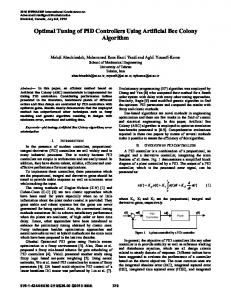
with khf = −60.7 dB. Fig. 6 and 7 show the frequency behavior of the resulting open loop system. As commented in the previous example, the fractional orders obtained in this case are significantly different from one (very far from the integer order controller performance). The corresponding step responses are given in Fig. 8 (for different gain values) and Fig. 9 (for different time constant values). C. Comments on the results

Fig. 4. Step response of the controlled system for L = 0 sec and different values of k

In both designs, the fractional (P I λ Dµ ) controllers perform in a robust way, taking into account the large parametric uncertainty and design specifications. As it can be seen in Fig. 2 and Fig. 6, the P I λ Dµ structure exhibits a rich frequency behavior, making the open loop gain fit closely to the stability boundary. Note that the optimal design should fit this stability boundary as close as possible, specially in the lower right corner. In contrast to other tuning techniques that guaranties

5405

Fig. 6.

Fig. 9. Step response of the controlled system for L = 5 sec and different values of τ

Bode diagram of the nominal open loop for L = 5 sec

nominal closed loop specifications, QFT guaranties the satisfaction of robust stability and performance specifications for all the considered parametric uncertainty. On the other hand, evolutionary algorithms have efficiently arrive to the given solution with a reasonable number of iterations, mainly due to the reduced number of parameter of the P I λ Dµ structure.

50 40 30

0.002

0.002

20 10 0

mag(L(jw)) (dB)

-10

V. C ONCLUSIONS

-20

λ

Tuning of P I D controllers has been recasted as a QFT loop shaping problem. This view of the tuning problem extends previous tuning techniques to consider robust control problems, where plant uncertainty is given in the form of QFT templates (including, for example, parametric uncertainty). This is a first work to analyze the potential of the P I λ Dµ controller to efficiently solve robust control problems. As a result, in comparison with other fractional structures previously used, P I λ Dµ controllers give a very good balance between complexity (number of parameters) and capacity to fit to frequency domain restrictions.

10

-30 -40 -50

-350

-300

-250

-200

-150

-100

-50

0

ang(L(jw)) (grados)

Fig. 7.

Nichols diagram of the nominal open loop for L = 5 sec

µ

VI. ACKNOWLEDGMENTS Work supported by the Projects 2PR02A0 (Junta Extremadura), MEC DPI2004-07670-C02-02 and 00507/PI/04 (Fundación Séneca, Murcia). R EFERENCES

Fig. 8. Step response of the controlled system for L = 5 sec and different values of k

[1] H. W. Bode, "Relations between Attenuation and Phase in Feedback Amplifier Design", Bell System Technical Journal, vol. 19, 1940, pp. 421-454. [2] H. W. Bode, Network Analysis and Feedback Amplifier Design. Van Nostrand, NY, 1945. [3] I. Horowitz, Quantitative Feedback Design Theory - QFT (Vol.1). QFT Press. Boulder, Colorado, USA, 1993. [4] S. Manabe, "The Non-Integer Integral and its Application to Control Systems", ETJ of Japan, vol. 6, no. 3-4, 1961, pp. 83-87. [5] A. Oustaloup, La Commande CRONE: Commande Robuste d’Ordre Non Entier, Hermes, Paris, 1991. [6] I. Podlubny, "Fractional-Order Systems and P I λ Dµ Controllers", IEEE Transactions on Automatic Control, vol. 44, 1999, pp. 208-214.

5406

[7] B. Vinagre, I. Podlubny, L. Dorcak, and V. Feliu, "On Fractional PID Controllers: A Frequency Domain Approach", in IFAC Workshop on Digital Control. Past, Present, and Future of PID Control, Terrasa, Spain, 2000, pp. 53-58. [8] R. Caponetto, L. Fortuna, and D. Porto, "A New Tuning Strategy for Non Integer Order PID Controller", in Proceedings of the First IFAC Workshop on Fractional Differentiation and Its Application, Bordeaux, France, 2004, pp. 168-173. [9] J. F. Leu, S. Y. Tsay, and C. Hwang, "Design of Optimal FractionalOrder PID Controllers", Journal of the Chinese Institute of Chemical Engineers, vol. 33, no. 2, 2002, pp. 193-202. [10] R. Barbosa, J. Tenreiro, and I. Ferreira, "Tuning of PID Controllers based on Bode’s Ideal Transfer Function", Nonlinear Dynamics, vol. 38, no. 1-4, 2004, pp. 305-321. [11] D.F. Thomson, Optimal and Sub-Optimal Loop Shaping in Quantitative Feedback Theory, School of Mechanical Engineering, Purdue University, West Lafayette, IN, USA, 1990. [12] A. Gera and I. Horowitz, "Optimization of the Loop Transfer Function", International Journal of Control, vol 31, 1980, pp. 389-398. [13] C. M. Frannson, B. Lenmartson, T. Wik, K. Holmström, M. Saunders and P. O. Gutman, "Global Controller Optimization Using Horowitz Bounds", in Proceedings of the IFAC 15th Trienial World Congress, Barcelona, Spain, 2002. [14] Y. Chait, Q. Chen, and C. V. Hollot, "Automatic Loop-Shaping of QFT Controllers via Linear Programming", ASME Journal of Dynamic Systems, Measurements and Control, vol. 121, 1999, pp. 351-357. [15] O. Yaniv and M. Nagurka, Automatic Loop Shaping of Structured Controllers Satisfying QFT Performance, Technical report, 2004. [16] W. H. Chen, D. J. Ballance, and Y. Li, Automatic Loop-Shaping of QFT using Genetic Algorithms, Center for Systems and Control, University of Glasgow, Glasgow, UK, 1998. [17] C. Raimúndez, A. Baños, and A. Barreiro, "QFT Controller Synthesis using Evolutive Strategies", in Proceedings of the 5th International QFT Symposium on Quantitative Feedback Theory and Robust Frequency Domain Methods, Pamplona, Spain, 2001, pp. 291-296. [18] J. Cervera and A. Baños, "Automatic Loop Shaping in QFT by using a Complex Fractional Order Terms Controller", in Proceedings of the 7th QFT and Robust Domain Methods Symposium, Pamplona, Spain, 2001, pp. 291-296. [19] J. Cervera and A. Baños, "Automatic Loop Shaping in QFT by using CRONE Structures", in Proceedings of the 2nd IFAC Workshop on Fractional Differentiation and Its Application, Porto, Portugal, 2006. [20] C. A. Monje, B. M. Vinagre, Y. Q. Chen, V. Feliu, P. Lanusse, and J. Sabatier, "Optimal Tuning for Fractional P I λ Dµ Controllers", in A. Le Mehauté, J. A. Tenreiro Machado, J. C. Trigeassou, and J. Sabatier (Eds.), Fractional Differentiation and its Application, Ubooks, Germany, 2006. [21] C. A. Monje, B. M. Vinagre, V. Feliu, and Y.Q. Chen, "On Auto-Tuning of Fractional Order P I λ Dµ Controllers", in Proceedings of the 2nd IFAC Workshop on Fractional Differentiation and Its Application, Porto, Portugal, 2006. [22] I. Horowitz, "Optimum Loop Transfer Function in Single-Loop Minimum-Phase Feedback Systems", International Journal of Control, vol. 18, 1973, pp. 97-113. [23] B. J. Lurie and P.J. Enright, Classical Feedback Control with MATLAB, Marcel Dekker, NY: 2000. [24] H. W. Bode, Network Analysis and Feedback Amplifier Design, Van Nostrand, NY: 1945. [25] C. A. Monje, Design Methods of Fractional Order Controllers for Industrial Applications, Ph.D Thesis, University of Extremadura, Badajoz, Spain, March 2006. [26] B. J. Lurie, "Tunable TID controller", US Patent 5.371,670,1994.

5407