IEEE TRANSACTIONS ON NEURAL NETWORKS, VOL. 17, NO. 1, JANUARY 2006
69
Tuning the Structure and Parameters of a Neural Network by Using Hybrid Taguchi-Genetic Algorithm Jinn-Tsong Tsai, Jyh-Horng Chou, Senior Member, IEEE, and Tung-Kuan Liu
Abstract—In this paper, a hybrid Taguchi-genetic algorithm (HTGA) is applied to solve the problem of tuning both network structure and parameters of a feedforward neural network. The HTGA approach is a method of combining the traditional genetic algorithm (TGA), which has a powerful global exploration capability, with the Taguchi method, which can exploit the optimum offspring. The Taguchi method is inserted between crossover and mutation operations of a TGA. Then, the systematic reasoning ability of the Taguchi method is incorporated in the crossover operations to select the better genes to achieve crossover, and consequently enhance the genetic algorithms. Therefore, the HTGA approach can be more robust, statistically sound, and quickly convergent. First, the authors evaluate the performance of the presented HTGA approach by studying some global numerical optimization problems. Then, the presented HTGA approach is effectively applied to solve three examples on forecasting the sunspot numbers, tuning the associative memory, and solving the XOR problem. The numbers of hidden nodes and the links of the feedforward neural network are chosen by increasing them from small numbers until the learning performance is good enough. As a result, a partially connected feedforward neural network can be obtained after tuning. This implies that the cost of implementation of the neural network can be reduced. In these studied problems of tuning both network structure and parameters of a feedforward neural network, there are many parameters and numerous local optima so that these studied problems are challenging enough for evaluating the performances of any proposed GA-based approaches. The computational experiments show that the presented HTGA approach can obtain better results than the existing method reported recently in the literature. Index Terms—Genetic algorithm (GA), neural networks (NN), Taguchi method.
I. INTRODUCTION
T
HE universal approximation capability of a neural network is one of the most exciting properties and has potentials for applications to problems such as system identification, communication channel equalization, signal processing, prediction, control, and pattern recognition [1]–[3]. A multilayer artificial neural network can approximate any nonlinear continuous function to an arbitrary accuracy [4]–[14]. Owing to its particular structure, a neural network is very good in learning using
Manuscript received March 5, 2004; revised March 7, 2005. This work was supported in part by the National Science Council, Taiwan, Republic of China, under Grant Numbers NSC93-2218-E327-001 and NSC93-2218-E037-001. J.-T. Tsai is with the Department of Medical Information Management, Kaohsiung Medical University, Kaohsiung 807, Taiwan, R.O.C. J.-H. Chou and T.-K. Liu are with the Department of Mechanical and Automation Engineering, National Kaohsiung First University of Science and Technology, Kaohsiung 824, Taiwan, R.O.C. (e-mail:
[email protected]). Digital Object Identifier 10.1109/TNN.2005.860885
some learning algorithms such as the genetic algorithm (GA) [15] and the backpropagation [16]. However, a fixed structure of overall connectivity between neurons may not provide the optimal performance within a given training period. A small network may not provide the good performance owing to its limited information processing power. A large network, on the other hand, may have some of its connections redundant [10], [17]–[19]. Therefore, recently, some researchers (for example, see [3], [10], [17]–[27], and references therein) have proposed various methods to solve the problem of learning the network structure and the connecting weights, where, in general, the network structure is considered to be a fully connected network as the number of the hidden nodes is fixed. Among the aforementioned works, Leung et al. [10], [19] particularly emphasized, after tuning, that a fully connected three-layer feedforward neural network could be reduced to a partially connected network as the number of the hidden nodes is fixed. In addition, among these researchers of studying the mentioned-above problem, Leung et al. [10], [19], Yao [18] Koza and Rice [20], Maniezzo [21], Zhang and Muhlenbein [22], Richards et al. [25], and Curran and O’Riordan [27] studied the problem of simultaneously tuning both network structure and parameters in a neural network by using the GA-based methods. In the works of Leung et al. [10], [19], the number of hidden nodes is manually chosen by increasing it from a small number until the learning performance in terms of fitness value is good enough. As a result, a fully connected three-layer network could be reduced to a partially connected network after tuning, as the number of the hidden nodes is fixed. This implies that the cost, in terms of hardware and processing time, of implementing the neural network can be reduced. In the problem of tuning both network structure and parameters simultaneously for a neural network, the particular challenge is that the GA-based methods may be trapped in the local optima of the objective function when the number of the parameters is large and there are numerous local optima. Therefore, the purpose of this paper is to apply a new robust approach, which is motivated by the work of the second author [28] of this paper and is named the hybrid Taguchi-genetic algorithm (HTGA) [29], to solve the problem of tuning both network structure and parameters of a feedforward neural network. The HTGA approach is a method of combining the traditional genetic algorithm (TGA) [15] with the Taguchi method [30]–[32]. In the HTGA approach, the Taguchi method is inserted between crossover and mutation operations of a TGA. Then, the systematic reasoning ability of the Taguchi method is incorporated
1045-9227/$20.00 © 2006 IEEE
70
IEEE TRANSACTIONS ON NEURAL NETWORKS, VOL. 17, NO. 1, JANUARY 2006
enough. Referring to Fig. 1, the input-output relationship of the MIMO three-layer feedforward neural network is as following:
(2.1) where
are the outputs which are functions of a variable are the inputs which are functions of a variable denotes the number of inputs; denotes the number of the hidden nodes; denotes the number of outputs; denotes the weight of the link between the th hidden node and the th denotes the weight of the link between the th output input; and denote the biases for the and the th hidden node; hidden nodes and output nodes, respectively; denotes the logarithmic sigmoid function: Fig. 1. Three-layer feedforward neural network.
(2.2) in the crossover operations to select the better genes to tailor the crossover operations in order to find the representative chromosomes to be the new potential offspring. Therefore, the Taguchi experimental design method can enhance the genetic algorithms, so that the HTGA approach can be more robust, statistically sound, and quickly convergent, where “more robust” means that the standard deviations of the fitness values are relatively small by using the presented HTGA approach. This paper is organized as follows. Section II describes the problem definition and the Taguchi method. The hybrid Taguchi-genetic algorithm for the three-layer feedforward neural network design is described in Section III. In Section IV, the authors first evaluate the performance of the applied HTGA approach and compare their results with those obtained from the improved-GA of Leung and Wang [33] for some well known test functions. Then, they use the HTGA approach to solve three examples on forecasting the sunspot numbers, tuning the associative memory, and solving the XOR problem. They also compare their results with those given by Leung et al. [10], [19] for the examples on forecasting the sunspot numbers and tuning the associative memory. Finally, Section V offers some conclusions.
II. PROBLEM DEFINITION AND TAGUCHI METHOD
As in [10], [19], , and denote the switches in links denotes that the th output is of the neural network. connected with the th hidden node, whereas denotes that the th output is not connected with the th hidden node. denotes that the th hidden node is connected with the th input, whereas denotes that the th hidden node is not connected with the th input. and denote that the biases are connected to the hidden and output layers, whereas and denote that the biases are not connected to the hidden and output layers, respectively. It can be seen that the weights of the links govern the input-output relationship of the neural network but the switches of the links govern the structure of the neural network. A number of the input and output neurons are fixed, but a number of the hidden neurons and the links between neurons are not fixed in the structure of the neural network. However, each input neuron at least has a connection to the hidden neuron and each hidden neuron at least has a connection to the output neuron. If the hidden neuron has no connection to the input neurons, the switch value in links of the neural network is equal to zero. The three-layer feedforward neural network can be employed to learn the input-output relationship of an application by using the HTGA approach. The input-output relationship of the MIMO three-layer feedforward neural network is described by (2.3)
In this section, the authors define the problem and describe the Taguchi method.
and are the given inputs and the desired , respectively; outputs of an unknown nonlinear function denotes the number of input-output pairs. The fitness function is defined as follows: where
A. Problem Definition The neural networks (NN) [3] for tuning usually have a fixed structure. The number of connections may be too large for a given application such that the network structure is unnecessarily complex and the implementation cost is high. In this paper, as the works of Leung et al. [10], [19], the authors consider a multiple-input-multiple-output (MIMO) three-layer feedforward neural network as shown in Fig. 1, and the number of hidden nodes is chosen by increasing it from a small number until the learning performance in terms of fitness value is good
(2.4) with
TSAI et al.: TUNING THE STRUCTURE AND PARAMETERS OF A NEURAL NETWORK
where the represents mean absolute error (MAE). The objective is to maximize the fitness value of (2.4). It can be seen from (2.4) that a larger fitness value implies a smaller error value. B. Taguchi Method Taguchi’s parameter design is an important tool for robust design. His tolerance design can be also classified as a robust design. Robust design is an engineering methodology for optimizing the product and process conditions which are minimally sensitive to the various causes of variation, and which produce high-quality products with low development and manufacturing costs. Two major tools used in the Taguchi method are the orthogonal array and the signal-to-noise ratio. Two-level orthogonal arrays are used in this paper. In this section, the authors briefly introduce the basic concept of the structure and use of two-level orthogonal arrays. Additional details and the detailed description of other-level orthogonal arrays can be found in the books presented by Phadke [30], Montgomery [31], and Park [32]. Many designed experiments use matrices called orthogonal arrays for determining which combinations of factor levels to use for each experimental run and for analyzing the data. In the past, orthogonal arrays were known as ‘Latin squares’ or ‘magic squares.’ Perhaps the effectiveness of orthogonal arrays in experimental design is magic. An orthogonal array is a fractional factorial matrix, which assures a balanced comparison of levels of any factor or interaction of factors. It is a matrix of numbers arranged in rows and columns where each row represents the level of the factors in each run, and each column represents a specific factor that can be changed from each run. The array is called orthogonal because all columns can be evaluated independently of one another. The general symbol for two-level standard orthogonal arrays is
of variation present and the mean response. There are several signal-to-noise ratios available depending on the type of characteristic: continuous or discrete; nominal-is-best, smaller-thebetter or larger-the-better. Here, the authors will only discuss the continuous case when the characteristic is smaller-the-better or larger-the-better. Further details can be found in the books presented by Phadke [30], Montgomery [31], and Park [32]. In the case of smaller-the-better characteristic, suppose that . Then the the authors have a set of characteristics natural estimate is
(2.6) where denotes the mean squared deviation from the target value of the quality characteristic, and the target value of is zero. Taguchi recommends using the common logarithm of this signal-to-noise ratio multiplied by 10, which expresses the ratio in decibels (dB); this has been used in communications for many years. To be consistent with its application in engineering, the is intended to be large for value of the signal-to-noise ratio favorable situations, and the authors use the following transformation for the smaller-the-better characteristic: (2.7) In the case of larger-the-better characteristic, similar to the smaller-the-better characteristic, the natural estimate is
(2.8)
(2.5) where = , the number of experimental runs; = positive integer which is greater than 1; = the number of levels for each factor; = the number of columns in the orthogonal array. The letter ‘ ’ comes from ‘Latin,’ the idea of using orthogonal arrays for experimental design having been associated with Latin square designs from the outset. The two-level standard orthogonal arrays most often used in practice are , and . In the field of communication engineering, a quantity called has been used as the quality characthe signal-to-noise ratio teristic of choice. Taguchi, whose background is communication and electronic engineering, introduced this same concept into the design of experiments. Two of the applications in which the concept of signal-to-noise ratio is useful are the improvement of quality via variability reduction and the improvement of measurement. The control factors that may contribute to reduced variation and improved quality can be identified by the amount of variation present and by the shift of mean response when there are repetitive data. The signal-to-noise ratio transforms several repetitions into one value, which reflects the amount
71
The corresponding signal-to-noise ratio becomes (2.9) which is also measured in decibels. Note that the target value of is zero in the larger-the-better characteristic. Example: Suppose the authors have two sets of five-quality and characteristic observations . The target value of is zero for the is also zero for smaller-the-better case. The target value of the larger-the-better case. Find the signal-to-noise ratios for each of two types of quality characteristic. Solution: a) Smaller-the-better case. From (2.7), the authors get that for the first set of data
(2.10a)
72
IEEE TRANSACTIONS ON NEURAL NETWORKS, VOL. 17, NO. 1, JANUARY 2006
and for the second set of data
(2.10b) b)
Larger-the-better case. From (2.9), the authors have that for the first set of data
(2.11a) and for the second set of data
in (3.1); and are where denotes the th element of the lower and the upper bounds of , respectively. Initialization procedure produces chromosomes, where denotes the population size, by the following algorithm. Algorithm: . Step 1) Generate a random value , where Step 2) Let . Repeat times and . produce a vector times and produce Step 3) Repeat the above steps initial feasible solutions. 2) Generation of Diversity Offspring by Crossover Operation: The crossover operators used here are one-cut-point operator integrated with arithmetical operator derived from convex set theory [15], [34], which randomly selects one cut-point, exchanges the right parts of two parents, and calculates the linear combinations in the cut-point genes to generate new offspring. For example, let two parents be and . If they are crossed after the th position, the resulting offspring are
(3.3) (2.11b) The larger the numerical value of (2.10) or (2.11) is, the more favorable the situation is. III. HTGA APPROACH FOR TUNING NEURAL NETWORK This section describes how to solve the problem of tuning both network structure and parameters of a three-layer feedforward neural network by using the HTGA approach. The details are as follows. 1) Generation of Initial Population: The real coding technique is applied to solve the problem of tuning both network structure and parameters of a neural network. In the real coding representation, each chromosome is encoded as a vector of floating numbers, with the same length as the vector of decision variables. For convenience and simplicity, let us denote (3.1), as shown at the bottom of the page, as the parameter vector of the three-layer feedforward neural network in (2.1), where is the number of total weights, biases, and switches with . In the practical application, the authors may have some other for some requirements. restrictions on the parameter vector The restrictions can be expressed as for or
for (3.2)
where and are the domain of , and is a random value, in which . and The crossover operators, , are only used to calculate the value of the weights or biases, whereas the value of the switches in the structure of neural network is determined based on whether the nodes are connected to each other. 3) Generation of the Better Offspring by Taguchi Method: The orthogonal arrays of the Taguchi method are used to study a large number of decision variables with a small number of experiments. The better combinations of decision variables are decided by the orthogonal arrays and the signal-to-noise ratios. The Taguchi concept is based on maximizing performance measures called signal-to-noise ratios by running a partial set of experiments using orthogonal arrays. In this study, a two-level orthogonal array is used. There are factors with two levels for each factor. To establish an orthogonal array of factors with two levels, let represent columns and individual experiments corresponding to is a positive integer , and the rows, where . If , the first columns are used and other columns are ignored. refers to the mean-square-deThe signal-to-noise ratio viation of objective function. Here, the authors modify (2.7) and (2.9) of the signal-to-noise ratios for this research. Let or if the objective function is to be maximized (larger-the-better) or minimized (smaller-the-better), denote the function evaluation value of respectively. Let experiment and , where is experiment times.
(3.1)
TSAI et al.: TUNING THE STRUCTURE AND PARAMETERS OF A NEURAL NETWORK
The effects of the various factors (variables) can be defined as following: sum of
for factor
at level
(3.4)
where is the experiment number, is the factor number, and is the level number. After crossover operation of the TGA, two chromosomes at a time are randomly chosen to execute matrix experiments of an orthogonal array. The primary goal in conducting a matrix experiment is to determine the best or the optimum level for each factor. The optimum level for a factor is the level that in the experimental region. For gives the highest value of , the optimum level is the the two-level problem, if level one for factor . Otherwise, level two is the optimum one. After the optimum level for each factor is selected, the optimum chromosome is also obtained. Therefore, the new offspring possesses the best or nearly the best function value among those of combinations of factor levels, which are all combinations of factor levels. 4) Mutation Operation: The basic concept of mutation operation is also derived from convex set theory [15], [34]. Two genes in a single chromosome are randomly chosen to execute the mutation of convex combination. For a given , if the elements and are randomly selected for mutation operation, the resulting . The two offspring is new genes and are and
(3.5)
. where is a random value and 5) Hybrid Taguchi-Genetic Algorithm: The HTGA approach is a method of combining the TGA with the Taguchi method. The Taguchi method is inserted between crossover and mutation operations of the TGA. Then, the systematic reasoning ability of the Taguchi method is incorporated in the crossover operations to select the better genes to achieve crossover, and consequently enhance the genetic algorithms. The steps of the HTGA approach are described as follows. Step 0) Parameter setting. Input: population size , crossover rate , mu, and number of generations. tation rate Output: the optimal chromosome and fitness value. Step 1) Initialization. Execute the Algorithm to generate an initial population. The fitness values of the population are then calculated. Step 2) Selection operation using the roulette wheel approach [35]. Step 3) Crossover operation. The probability of crossover is determined by crossover rate . Step 4) Select a suitable two-level orthogonal array for matrix experiments. The orthogonal arrays , and are used to test the examples given in the next section. Step 5) Choose randomly two chromosomes at a time to execute matrix experiments.
73
Step 6) Calculate the fitness values and signal-to-noise ratios of experiments in the orthogonal array . Step 7) Calculate the effects of the various factors ( and ). Step 8) One optimal chromosome is generated based on the results from Step 7). Step 9) Repeat Steps 5) through 8) until the expected has been met. number Step 10) The population via the Taguchi method is generated. Step 11) Mutation operation. The probability of mutation is . determined by mutation rate Step 12) Offspring population is generated. Step 13) Sort the fitness values in increasing order among parents and offspring populations. chromosomes as parents of the Step 14) Select the better next generation. Step 15) Has the stopping criterion been met? If yes, then go to Step 16). Otherwise, return to Step 2) and continue through Step 15). Step 16) Display the optimal chromosome and the fitness value. IV. DESIGN EXAMPLES AND COMPARISONS First, in this section, in order to make this paper more complete, the authors adopt the partial results of their works [28], [29] regarding the HTGA approach to show the performance of the presented HTGA approach. Here, the authors use the presented HTGA approach to solve the global numerical optimization problems, evaluate the performance of the presented HTGA approach, and compare their results with those given by Leung and Wang [33] for some well known test functions in Table I, where the authors use the same evolutionary parameters as those adopted by Leung and Wang [33]. The algorithm presented by Leung and Wang [33], which is named the orthogonal genetic algorithm with quantization (OGA/Q), not only can find optimal or close-to-optimal solutions but also can give more robust and significantly better results than those other improved-GAs presented by Renders and Bersini [36], Michalewicz [37], Yen and Lee [38], and Chellapilla [39]. Second, the authors adopt the same examples as those considered by Leung et al. [10], [19] to test their presented HTGA approach, and to compare the performance of their presented HTGA approach with that of the GA-based approach given by Leung et al. [10], [19], where they adopt the same population size and the same number of iterations as those used by Leung et al. [10]. Third, the HTGA approach is applied to solve the XOR problem for tuning both the connection weights and the number of the connection links in the three-layer neural network. A. Solving the Global Numerical Optimization Problems In this section, the authors execute their presented HTGA approach to solve these test functions in Table I with 30 dimensions (i.e., ) for functions . In this manner, these test functions have so many local minima that they
74
IEEE TRANSACTIONS ON NEURAL NETWORKS, VOL. 17, NO. 1, JANUARY 2006
TABLE I TEST FUNCTIONS
are challenging enough for performance evaluation, and the existing results reported by Leung and Wang [33] can be used for a direct comparison. In the work of Leung and Wang [33], the following evolutionary environments are used: 1) the population size is 200; 2) the crossover rate is 0.1; and 3) the mutation rate is 0.02. Each test function was performed in 50 independent runs and the following results were recorded: i) the mean number of function evaluations; ii) the mean function value (i.e., the mean of the function values was found in the 50 runs); and iii) the standard deviation of the function values. In the computational experiments of the presented HTGA approach, the HTGA approach uses the same evolutionary parameters as those adopted by the OGA/Q. The authors set up the stopping criterion under which the execution of the algorithm of the presented HTGA would be stopped as soon as the smallest function value of the fitness member of the population is less than or equal to the mean function value given by the OGA/Q. In addition, each test function is performed with 50 independent runs. The mean number of function evaluations, the mean function value, and the standard deviation of the function values are all recorded for each test function. Table II shows the performance comparisons between the presented HTGA and the OGA/Q given by Leung and Wang [33] under the same evolutionary environments [29]. Here, the authors discuss the analysis of complexity by using the results of this example instead of the theory of Vapnik-Chervonenkis dimension [40]. From the fewer mean numbers of function evaluations and more stable solution quality, it can be seen that, from Table II, the HTGA approach compared with other GA-based methods has a lower computational time requirement, though it is not proved by the serious mathematical viewpoint. From
Table II, it can be seen that i) the presented HTGA can find optimal or close-to-optimal solutions; , and , the presented HTGA can give better ii) for and closer-to-optimal solutions than the OGA/Q, and , and , both HTGA and OGA/Q can give for the same optimal or close-to-optimal solutions; iii) the presented HTGA gives smaller standard deviations of function values than the OGA/Q, and hence the presented HTGA has a more stable solution quality; iv) the presented HTGA requires fewer mean numbers of function evaluations than the OGA/Q, and hence the proposed HTGA has a lower computational time requirement. Furthermore, the execution of the presented HTGA can be stopped for each run under the stopping criterion, so that the standard deviation of function values for each function is zero. In other words, these results in Table II indicate that the presented HTGA can give better mean solution quality and more stable solution quality than the OGA/Q. In addition, the HTGA approach is also better than those improved-GAs methods presented by Renders and Bersini [36], Michalewicz [37], Yen and Lee [38], and Chellapilla [39], because that the OGA/Q approach has been shown to be better than those improved-GAs methods presented by Renders and Bersini [36], Michalewicz [37], Yen and Lee [38], and Chellapilla [39]. The additional comparisons and discussions on the other test functions can be found in the works given by the authors of this paper [28], [29]. Hence, the authors could conclude that the presented HTGA approach is very feasible to solve the global numerical optimization problems. After the above demonstrating of capability for the HTGA approach, the authors use the HTGA approach
TSAI et al.: TUNING THE STRUCTURE AND PARAMETERS OF A NEURAL NETWORK
75
TABLE II COMPARISONS BETWEEN HTGA AND OGA/Q UNDER THE SAME EVOLUTIONARY ENVIRONMENTS
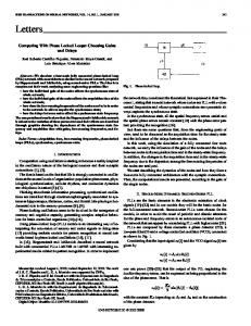
Fig. 2. Sunspot cycles from year 1700 to 1980.
to solve three examples on forecasting the sunspot numbers, tuning the associative memory, and solving the XOR problem for tuning both parameters and structure of the three-layer feedforward neural network. B. Forecasting of the Sunspot Numbers An application example on forecasting the sunspot numbers [1], [10], [19], [41] is given in this section. The sunspot cycles
from year 1700 to 1980 are shown in Fig. 2. The maximum sunspot number is 200 between year 1700 and 1980. The cycles generated are nonlinear, nonstationary, and non-Gaussian which are difficult to model and predict. The three-layer feedforward three-input-single-output neural network is used for the sunspot , of the neural network numbers forecasting. The inputs, , are defined as , where denotes the year and and is the sunspot number at the year . The sunspot numbers of the
76
IEEE TRANSACTIONS ON NEURAL NETWORKS, VOL. 17, NO. 1, JANUARY 2006
TABLE III RESULTS OF FITNESS VALUES FOR THE EXAMPLE ON FORECASTING THE SUNSPOT NUMBERS BY USING THE HTGA APPROACH
first 180 years (i.e., ) are used to train the neural network. Referring to (2.1), the neural network used for the sunspot numbers forecasting is governed by
(4.1) In order to obtain the optimal network structure, the algorithm is starts with a small network. The number of hidden nodes increased from four to eight and the number of the connection links is chosen by increasing it from a small number until the learning performance of network is good enough. In addition, is given as the fitness function is defined in (2.4), where the following:
and thus it is very robust. From the computational results in Table IV, it can be seen that, for each of the same number of the hidden nodes, the presented HTGA approach can give the better fitness values and fewer links than the GA-based method given by Leung et al. [10], [19]. Referring to Table IV, the best result is obtained by using the HTGA approach when the number of hidden node is five. The number of connection links is eight after learning (the number of links of a fully connected network is 26 which includes the bias links). It is about 70% reduction of links. The training error and the forecasting error are 9.146 55 and 13.797 72, respectively. Hence, the authors could conclude that the HTGA approach has a good performance on tuning both parameters and structure of the three-layer feedforward neural network for the example on forecasting the sunspot numbers. C. Associative Memory Another application example on tuning an associative memory is given in this section. In this example, the associative memory, which maps its input vector into itself, has ten inputs and ten outputs. Thus, the desired output vector is its input vector. Fifty input vectors provided by Leung et al. [10], [19] are used to test the learning performance. Referring to (2.1), the three-layer feedforward neural network used for the associative memory is given by
(4.3) The fitness function is defined in (2.4), where the following:
is given as
(4.2)
(4.4)
The HTGA approach is employed to tune the parameters and structure of the three-layer neural network in (4.1). The objective is to maximize the fitness function. The best fitness value is one and the worst one is zero. In this example, the lower and , and are assumed to be the upper bounds of and 100, respectively. The switch value of , and is defined to be zero or one, depending on the link connection or not. The following evolutionary environments are used by the presented HTGA approach in this example: the crossover rate is 0.9, and the mutation rate is 0.1. The best fitness value, the average fitness value, and the standard deviation among 20 runs for the example on forecasting the sunspot numbers by using the presented HTGA approach are shown in Table III. trainingerror , the The fitness value defined by training error defined by , the , and forecasting error defined by the number of links are tabulated in Table IV. The computational results obtained by using the presented HTGA approach and the GA-based method given by Leung et al. [10], [19], respectively, are given in Table IV. From Table III, it can be seen that the presented HTGA approach gives very small standard deviations of fitness values,
The HTGA approach is used to tune the parameters and structure of the three-layer neural network in (4.3). The objective is to maximize the fitness function. The best fitness value is one and the worst one is zero. Here, all parameters in (4.3) are assumed to be in the same region as that considered in the example on forecasting the sunspot numbers. In this example, there are many parameters and numerous local optima so that this studied problem is challenging enough for evaluating the performance of the presented HTGA approach and that of the GA-based method proposed by Leung et al. [10], [19]. In this example, the following evolutionary environments are used by the presented HTGA approach: The crossover rate is 0.9, and the mutation rate is 0.1. The best fitness value, the average fitness value, and the standard deviation among 20 runs for the example on tuning an associative memory by using the presented HTGA approach are shown in Table V. The computational results obtained by using the presented HTGA approach and the GA-based method given by Leung et al. [10], [19] are given in Table VI. From Table V, it can be seen that the presented HTGA approach gives small standard deviations of fitness values, and thus it is very robust. From the computational results in Table VI, it can be seen that, for each of the same number of the hidden
TSAI et al.: TUNING THE STRUCTURE AND PARAMETERS OF A NEURAL NETWORK
77
TABLE IV COMPUTATIONAL RESULTS FOR THE EXAMPLE ON FORECASTING THE SUNSPOT NUMBERS
TABLE V RESULTS OF FITNESS VALUES FOR THE EXAMPLE ON TUNING AN ASSOCIATIVE MEMORY BY USING THE HTGA APPROACH
nodes, the presented HTGA approach can give the better fitness values and fewer links than the GA-based approach given by Leung et al. [10], [19]. In order to obtain the optimal network structure, the algorithm starts with a small network. The is increased from four to eight and number of hidden nodes the number of the connection links is chosen by increasing it from a small number until the learning performance of network is good enough. Referring to Table VI, the best result is obtained by using the HTGA approach when the number of hidden node is seven. The number of connected link is 60 after learning (the number of links of a fully connected network is 157 which includes the bias links). It is about 62% reduction of links. In addition, it can be seen from Table VI that the HTGA approach can find the feasible parameters to fit the requirements of tuning an associative memory having only 60 links for the neural network with the different hidden nodes. Hence, the authors could conclude that the HTGA approach can find a smaller neural network for the example on tuning an associative memory. In addition, the authors also provide the comparison of results obtained by the GA with and without Taguchi method. For example, in the case of the same evolutionary environments as those mentioned above, four hidden nodes and 60 links for the network,
the training time for the network, with and without Taguchi method, is roughly 40 seconds by using the computer of 1.8 GHz CPU with 256 Mb RAM under the same number (for example, 22 550) of fitness evaluations. The viewpoint of the computation time is not concerned, because it depends on the computer machine of the different hardware specifications and operation system, the programming language, the individual skill of programming, and so on. The main point the authors concern is the final fitness values with and without Taguchi method under the same network and the same number of fitness evaluations. In this case, the final fitness values with and without Taguchi method are 0.9674 and 0.9433, respectively, under the aforementioned same conditions. That is, the GA with Taguchi method has a better search capability than the GA without Taguchi method. D. XOR Problem The XOR logic function has two inputs and one output. It produces an output only if either one or the other of the inputs is on, but not if both are off or both are on. the authors consider this as a problem that the authors apply the presented HTGA is on and approach to solve: The output is one when the is off, or when the is on and is off; otherwise the output is zero. The neural network is of size 2-2-1, that is, two neurons in the input layer, two neurons in the hidden layer, and one neuron in the output layer. The objective by using the HTGA approach is to tune the connection weights and the number of the connection links of the neural network, and to produce the desired classifications for the XOR inputs. The XOR problem solved by the back-propagation network is of nine variables (connection links) in the network: four weights connecting the input to hidden nodes, two weights connecting the hidden to outputs, and three thresholds. However, the HTGA approach can find the feasible connection weights to produce the desired classifications having only six links of connection
78
IEEE TRANSACTIONS ON NEURAL NETWORKS, VOL. 17, NO. 1, JANUARY 2006
TABLE VI COMPUTATIONAL RESULTS FOR THE EXAMPLE ON TUNING AN ASSOCIATIVE MEMORY
Fig. 3. Neural network of six connection links for the XOR problem.
for the neural network as shown in Fig. 3. The neural network for the XOR problem is governed by (4.5) is defined in (2.2). In the classification where process, if , the output is one when the is on and is off, or when the is on and is off; if , the output is zero when both are off or both are on. One set of the weights for the successful classification is , where is shown in Fig. 3. Therefore, it can be seen that, from the aforementioned result, the presented HTGA approach can use a smaller neural network for classifications in the XOR problem. V. CONCLUSION In this paper, the HTGA approach has been applied to solve the tuning problem of both structure and parameters of the three-layer feedforward neural network. The HTGA approach is a method of combining the TGA, which have the merit of powerful global exploration capability, with the Taguchi method, which can exploit the optimum offspring.
The two-level orthogonal array and the signal-to-noise ratio of the Taguchi method are used for exploitation. The optimum chromosome can be easily found by using both experimental runs and signal-to-noise ratios instead of executing combinations of factor levels, which are all combinations of factor levels. Moreover, the Taguchi method is also a robust design approach, which draws on many ideas from statistical experimental design to plan experiments for obtaining dependable information about variables, so it can achieve the population distribution closest to the target and make the results robust. In the presented HTGA approach, the Taguchi method is inserted between crossover and mutation operations of the TGA. Then, the systematic reasoning ability of the Taguchi method is incorporated in the crossover operations to select the better genes to achieve crossover, and consequently enhance the genetic algorithms. The authors use the HTGA approach to solve the benchmark problems with 30 dimensions. The computational experiments show that the presented HTGA approach can find optimal or close-to-optimal solutions, and it is more efficient than the OGA/Q proposed by Leung and Wang [33] on the problems studied. Therefore, the presented HTGA approach possesses the merits of global exploration, fast convergence, robustness, and statistical soundness [28], [29]. Furthermore, the authors applied the introduced HTGA approach to solve three examples on forecasting the sunspot numbers, tuning an associative memory, and solving the XOR problem. As a result, a given fully connected three-layer neural network can be reduced to a partially connected network after learning. This implies that the cost, in terms of hardware and processing time, of implementing the compact neural network can be reduced. In these studied problems on forecasting the sunspot numbers and tuning an associative memory, there are many parameters and numerous local optima so that these studied problems are challenging enough for evaluating the performance of the presented HTGA approach and that of the GA-based approach
TSAI et al.: TUNING THE STRUCTURE AND PARAMETERS OF A NEURAL NETWORK
proposed by Leung et al. [10], [19]. The computational experiments show that the presented HTGA approach can obtain better results than the GA-based method given by Leung et al. [10], [19]. In addition, the HTGA approach also can use a smaller neural network for classifications in the XOR problem. ACKNOWLEDGMENT The authors would like to thank Dr. H. K. Lam, who is with the Department of Electronic and Information Engineering at the Hong Kong Polytechnic University, for his help in the period of this research. The authors would also like to thank the Associate Editor and referees for their constructive and helpful comments and suggestions. REFERENCES [1] M. Li, K. Mechrotra, C. Mohan, and S. Ranka, “Sunspot numbers forecasting using neural network,” in Proc. 5th IEEE Int. Symp. Intelligent Control, Philadelphia, PA, 1990, pp. 524–528. [2] M. Brown and C. Harris, Neural Fuzzy Adaptive Modeling and Control. Englewood Cliffs, NJ: Prentice-Hall, 1994. [3] M. M. Gupta, L. Jin, and N. Homma, Static and Dynamic Neural Networks, New York: Wiley, 2003. [4] R. Hecht-Neilsen, “Kolmogorov mapping neural network existence theorem,” in Proc. IEEE First Int. Conf. Neural Networks, San Diego, CA, 1987, pp. 11–13. [5] B. Irie and S. Miyake, “Capabilities of three-layered perceptrons,” in Proc. IEEE Int. Conf. Neural Networks, San Diego, CA, 1988, pp. 641–648. [6] K. I. Funahashi, “On the approximate realization of continuous mappings by neural networks,” Neural Netw., vol. 2, pp. 183–192, 1989. [7] K. Hornick, M. Stinchcombe, and H. White, “Multilayer feedforward networks are universal approximators,” Neural Netw., vol. 2, pp. 359–366, 1989. [8] D. A. Vaccari and E. Wojciechowski, “Neural networks as function approximators: Teaching a neural network to multiply,” in Proc. 1994 IEEE Int. Conf. Neural Networks: IEEE World Congr. Computational Intelligence, Orlando, FL, 1994, pp. 2217–2222. [9] D. Tien and P. Nobar, “Dificiency in the current trend of training of neural network systems, suggestions and solutions,” in Proc. IEEE Region 10 Int. Conf. Electrical and Electronic Technology, Singapore, 2001, pp. 43–49. [10] H. F. Leung, H. K. Lam, S. H. Ling, and K. S. Tam, “Tuning of the structure and parameters of a neural network using an improved genetic algorithm,” IEEE Trans. Neural Netw., vol. 14, no. 1, pp. 79–88, Jan. 2003. [11] S. Ferrari, M. Maggioni, and N. A. Borghese, “Multiscale approximation with hierarchical radial basis functions networks,” IEEE Trans. Neural Netw., vol. 15, no. 1, pp. 178–188, Jan. 2004. [12] P. Y. Liu and H. X. Li, “Efficient learning algorithms for three-layer regular feedforward fuzzy neural networks,” IEEE Trans. Neural Netw., vol. 15, no. 3, pp. 545–558, May 2004. [13] S. Ferrari and R. F. Stengel, “Smooth function approximation using neural networks,” IEEE Trans. Neural Netw., vol. 16, no. 1, pp. 24–38, Jan. 2005. [14] G. B. Huang, P. Saratchandran, and N. Sundararajan, “A generalized growing and pruning RBF (GGAP-RBF) neural network for function approximation,” IEEE Trans. Neural Netw., vol. 16, no. 1, pp. 57–67, Jan. 2005. [15] M. Gen and R. Cheng, Genetic Algorithms and Engineering Design. New York: Wiley, 1997. [16] D. T. Pham and D. Karaboga, Intelligent Optimization Techniques: Genetic Algorithms, Tabu Search, Simulated Annealing and Neural Networks. New York: Springer-Verlag, 2000.
79
[17] X. Yao and Y. Liu, “A new evolutionary system for evolving artificial neural networks,” IEEE Trans. Neural Netw., vol. 8, no. 3, pp. 694–713, 1997. [18] X. Yao, “Evolving artificial networks,” Proc. IEEE, vol. 87, pp. 1423–1447, 1999. [19] H. F. Leung, H. K. Lam, S. H. Ling, and K. S. Tam, “Tuning of the structure and parameters of neural network using an improved genetic algorithm,” Proc. 27th Annu. Conf. IEEE Industrial Electronics Society, pp. 25–30, 2001. [20] J. R. Koza and J. P. Rice, “Genetic generation of both the weights and architecture for a neural network,” in Proc. Int. Joint Conf. Neural Networks, Seattle, WA, 1991, pp. 397–404. [21] V. Maniezzo, Searching Among Search Spaces: Hastening the Genetic Evolution of Feedforward Neural Networks. New York: Springer-Verlag, 1993. [22] B. Zhang and H. Muhlenbein, “Evolving optimal neural networks using genetic algorithms with occam’s razor,” Complex Systems, vol. 7, pp. 199–229, 1993. [23] Y. Q. Chen, D. W. Thomas, and M. S. Nixon, “Generating-shrinking algorithms for learning arbitrary classification,” Neural Netw., vol. 7, pp. 1477–1489, 1994. [24] C. C. Teng and B. W. Wah, “Automated learning for reducing the configuration of a feedforward neural network,” IEEE Trans. Neural Netw., vol. 7, no. 5, pp. 1072–1085, Sep. 1996. [25] N. Richards, D. E. Moriarty, and R. Miikkulainen, “Evolving neural networks to play go,” Applied Intelligence, vol. 8, pp. 85–96, 1997. [26] N. K. Treadgold and T. D. Gedeon, “Exploring constructive cascade networks,” IEEE Trans. Neural Netw., vol. 10, no. Nov., pp. 1335–1350, 1997. [27] D. Curran and C. O’Riordan, “Applying Evolutionary Computation to Designing Neural Networks: A Study of the State of the Art,” Department of Information Technology, National University of Ireland, Galway, Ireland, Technical Report NUIG-IT-111 002, 2002. [28] J. H. Chou, W. H. Liao, and J. J. Li, “Application of Taguchi-genetic method to design optimal grey-fuzzy controller of a constant turning force system,” in Proc. 15th CSME Annu. Conf., Tainan, Taiwan, 1998, pp. 31–38. [29] J. T. Tsai, T. K. Liu, and J. H. Chou, “Hybrid Taguchi-genetic algorithm for global numerical optimization,” IEEE Trans. Evol. Comput., vol. 8, no. 4, pp. 365–377, Aug. 2004. [30] M. S. Phadke, Quality Engineering Using Robust Design. Englewood Cliffs, NJ: Prentice-Hall, 1989. [31] D. C. Montgomery, Design and Analysis of Experiments. New York: Wiley, 1991. [32] S. H. Park, Robust Design and Analysis for Quality Engineering. London, U.K.: Chapman & Hall, 1996. [33] Y. W. Leung and Y. Wang, “An orthogonal genetic algorithm with quantization for global numerical optimization,” IEEE Trans. Evol. Comput., vol. 5, no. 1, pp. 41–53, Feb. 2001. [34] M. Bazaraa, J. Jarvis, and H. Sherali, Linear Programming and Network Flows. New York: Wiley, 1990. [35] D. E. Goldberg, Genetic Algorithms in Search, Optimization and Machine Learning, MA: Addison-Wesley, 1989. [36] J. Renders and H. Bersini, “Hybridizing genetic algorithms with hillclimbing methods for global optimization: Two possible ways,” Proc. First IEEE Conf. Evolutionary Computation , pp. 312–317, 1994. [37] Z. Michalewicz, Genetic Algorithms Data Structures Evolution Programs. Berlin, Germany: Springer-Verlag, 1996. [38] J. Yen and B. Lee, “A simplex genetic algorithm hybrid,” in Proc. IEEE Int. Conf. Evolutionary Computation , Indianapolis, IN, 1997, pp. 175–180. [39] K. Chellapilla, “Combining mutation operators in evolutionary programming,” IEEE Trans. Evol. Comput., vol. 2, no. 3, pp. 91–96, Sep. 1998. [40] The Handbook of Brain Theory and Neural Networks, M. A. Arbib, Ed., MIT Press, MA, 1995, pp. 1000–1003. W. Maass, Vapnik-Chervonenkis Dimension of Neural Nets. [41] T. J. Cholewo and J. M. Zurada, “Sequential network construction for time series prediction,” in Proc. Int. Conf. Neural Networks, Houston, TX, 1997, pp. 2034–2038.
+
=
80
Jinn-Tsong Tsai received the B.S. and the M.S. degrees in mechanical engineering from National Sun Yat-Sen University, Taiwan, in June 1986 and June 1988, respectively, and the Ph.D. degree in engineering science and technology from National Kaohsiung First University of Science and Technology, Taiwan, in June 2004. He is currently an Assistant Professor of Medical Information Management Department at Kaohsiung Medical University, Taiwan. From July 1988 to May 1990, he was a Lecturer at the Vehicle Engineering Department, Chung Cheng Institute of Technology, Taiwan. From July 1990 to August 2004, he was a Researcher and the Chief of Automation Control Section at Metal Industries Research and Development Center, Taiwan. His research interests include evolutionary computation, intelligent control and systems, neural networks, and quality engineering.
Jyh-Horng Chou (M’04–SM’04) received the B.S. and the M.S. degrees in engineering science from National Cheng-Kung University, Taiwan, in June 1981 and June 1983, respectively, and the Ph.D. degree in mechatronic engineering from National Sun Yat-Sen University, Taiwan, in December 1988. He is currently a Professor and the Vice President at the National Kaohsiung First University of Science and Technology, Taiwan. From August 1983 to July 1986, he was a Lecturer at the Mechanical Engineering Department, National Sun Yat-Sen University, Taiwan. From August 1986 to July 1991, he was an Associate Professor at the Mechanical Engineering Department and the Director of the Center for Automation Technology, National Kaohsiung University of Applied Sciences, Taiwan. From August 1991 to July 1999, he was a Professor and the Chairman of Mechanical Engineering Department at National Yunlin University of Science and Technology, Taiwan. From August 1999 to September 2004, he was a Professor and Chairman at the Mechanical and Automation Engineering Department, and from October 2004 to December 2005, he was a Professor and the Dean of Engineering College at National Kaohsiung First University of Science and Technology, Taiwan. He has coauthored three books and published more than 155 refereed journal papers and 135 conference papers. He also holds two patents (one is in the technology area of automation, and the other one is in the area of computational intelligence). His research and teaching interests include intelligent systems and control, computational intelligence and methods, robust control, and quality engineering. Dr. Chou received both the Research Award and the Excellent Research Award from the National Science Council of Taiwan fourteen times. He also received the 2004 Excellent Project Outcome Award of the Educational Promotion Project on the Integrated Manufacturing and e-Commerce Technology from the Ministry of Education, Taiwan, the 2005 Outstanding Research Award from National Kaohsiung First University of Science and Technology, Taiwan, and the 2005 Outstanding Achievement Award for alumnus graduated from Engineering Science Department at National Cheng-Kung University, Taiwan. He is currently an Editorial Member for the Journal of the Chinese Society of Mechanical Engineers, and an Associate Editor for the International Journal of Information and Systems Sciences.
Tung-Kuan Liu received the B.S. degree in mechanical engineering from National Akita University, Japan, in March 1992 and the M.S. and the Ph.D. degrees in mechanical engineering and information science from National Tohoku University, Japan, in March 1994 and March 1997, respectively. He is currently an Associate Professor at the Mechanical and Automation Engineering Department, National Kaohsiung First University of Science and Technology, Taiwan. From October 1997 to July 1999, he was a Senior Manager at the Institute of Information Industry, Taiwan. From August 1999 to July 2002, he was also an Assistant Professor at the Department of Marketing and Distribution Management, National Kaohsiung First University of Science and Technology, Taiwan. His research and teaching interests include artificial intelligence, applications of multi-objective optimization genetic algorithms, and integrated manufacturing and business systems.
IEEE TRANSACTIONS ON NEURAL NETWORKS, VOL. 17, NO. 1, JANUARY 2006