Neural-network-based Variable Structure Control Of ... - IEEE Xplore

50

IEEE/ASME TRANSACTIONS ON MECHATRONICS, VOL. 4, NO. 1, MARCH 1999

Neural-Network-Based Variable Structure Control of Electrohydraulic Servosystems Subject to Huge Uncertainties Without Persistent Excitation Chih-Lyang Hwang, Associate Member, IEEE

Abstract—A novel scheme investigating a radial-basis-function neural network (RBFNN) with variable structure control (VSC) for electrohydraulic servosystems subject to huge uncertainties is presented. Although the VSC possesses some advantages (e.g., fast response, less sensitive to uncertainties, and easy implementation), the chattering control input often occurs. The reason for a chattering control input is that the switching control in the VSC is used to cope with the uncertainties. The larger the uncertainties which arise, the larger switching control occurs. In this paper, an RBFNN is employed to model the uncertainties caused by parameter variations, friction, external load, and controller. A new weight updating law using a revision of e-modification by a timevarying dead zone can achieve an exponential stability without the assumption of persistent excitation for the uncertainties or radial basis function. Then, an RBFNN-based VSC is constructed such that some part of uncertainties are tackled, that the tracking performance is improved, and that the level of chattering control input is attenuated. Finally, the stability of the overall system is verified by the Lyapunov stability criterion. Index Terms— Electrohydraulic servosystems, persistent excitation, radial-basis-function neural network, variable structure control.

I. INTRODUCTION

T

HE development of reliable electrohydraulic elements interfaced to microcontrollers has been the most significant factor in the renaissance of the hydraulic systems. The electrohydraulic servovalves serve as interfaces between the electrical devices and the hydraulic system. They are capable of converting the low-power electrical inputs into the movement of spools to precisely control a large-power low-speed hydraulic actuator. For instance, they are used extensively in such applications as computer numerical control machine tools, aircraft, ship steering gear, and test machinery [1]–[5]. However, some nonlinear time-varying phenomena, such as the relationship between input current and output flow, fluid compressibility, deadband due to the internal leakage and hysteresis, friction in the cylinder (or hydraulic motor), and external load [6], [7], make the control or modeling of hydraulic systems difficult.

Manuscript received July 14, 1997; revised February 11, 1998 and June 12, 1998. Recommended by Technical Editor K. Ohnishi. This work was supported in part by the National Science Council of Taiwan, R.O.C., under Grant NSC-87-2218-E-036-001. The author is with the Department of Mechanical Engineering, Tatung Institute of Technology, Taipei, 10451 Taiwan, R.O.C. Publisher Item Identifier S 1083-4435(99)02311-X.

The controller designs for these control systems can be variable structure control (VSC) (e.g., [8] and [9]), adaptive control (e.g., [10] and [11]), and fuzzy control. The distinct controller has its own advantages and disadvantages. Although VSC provides a robust means for controlling a nonlinear dynamic system with uncertainties, it always results in a chattering control input due to its discontinuous switching control used to deal with the uncertainties. The larger the uncertainties which take place, the larger is the switching control which occurs. The chattering control input has some drawbacks, e.g., easy damage of mechanism and excitation of unmodeled dynamics. Hence, how to obtain a chattering-free VSC with an acceptable tracking result for the electrohydraulic servosystems subject to enormous uncertainties becomes an important topic. The most commonly used method for attenuating the chattering control input is the boundary layer method [12]–[15]. Indeed, the control input is smoother than that without using a boundary layer. However, its stability is guaranteed only outside of the boundary layer, and its tracking error is bounded by the width of boundary layer [12]–[15]. In this paper, a radial-basis-function neural network (RBFNN) is employed to model the uncertainties caused by parameter variations, friction, external load, and controller. Then, an RBFNN-based VSC with time-varying switching gain and boundary layer [9] is designed such that some part of the uncertainties are tackled, that the tracking performance is improved, and that the level of chattering control input is attenuated. The reason to use an RBFNN but not to use another neural network (e.g., multilayer neural network [16]) is that the RBFNN results in the nonlinear maps in which the connection weights occur linearly. Hence, the stability of the overall system is not difficult to accomplish, the updating law for adjusting is substantially simplified, and the convergence of connection weights is rapid [7], [17]–[19]. Furthermore, many papers examine the neuro control or neural network modeling for nonlinear systems [20]–[23]. Numerous papers discussing adaptive control for the system in the presence of disturbances were given one or two decades ago. For example, a dead zone in the adaptive law [24]–[26] guarantees the boundedness of all the signals in the adaptive loop. In addition, [24], as well as [26], restrict the search region of parameter space by using a priori information about the in the bound of parameter. An extra term of the form adaptive law for adjusting the parameter introduced in [27] is referred to as -modification. In [28], an -modification

1083–4435/99$10.00  1999 IEEE

HWANG: NEURAL-NETWORK-BASED VARIABLE STRUCTURE CONTROL OF ELECTROHYDRAULIC SERVOSYSTEMS

51

is designed to improve the performance of the system in all respects, while retaining the advantage of assuring robustness in the presence of disturbances without the requirement of persistent excitation (PE). In this paper, a revision of modification using a time-varying dead zone is employed to achieve an exponential stability without the assumption of PE for the uncertainties. Whatever the uncertainties which occur, its assumption about PE is not assigned so that the controller design is more practical because of the difficulty of satisfying the PE condition in an RBFNN [29]. Hence, without the assumption of PE [16], [29], the proposed updating law can force the connection weights of the RBFNN into the vicinity of their optimal values. Together with the robustness of VSC, the control performance of an electrohydraulic servosystem in the presence of huge uncertainties is excellent. II. PROBLEM FORMULATION

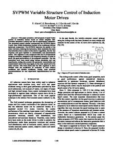
Fig. 1. The control block diagram of the overall system.

First, the dynamics of an electrohydraulic servosystem is considered as follows. The relationship between the servovalve (m) and the load flow (m /s) is displacement described in the following servovalve equation:

where is the servovalve gain. Define the following state variables:

(1) denotes the servovalve flow-pressure coefficient where stands for the load differential pressure (m /s/MPa), is called the servovalve flow gain, given by (MPa), and

(7) Then, the state variable equation describing the dynamics of the electrohydraulic servosystems is achieved as follows:

(2) denotes the discharge coefficient (dimensionless), where is the area of gradient (m), represents the fluid mass is the supply pressure (Mpa). The density (kg/m ) and continuity equation to the hydraulic motor chamber gives

(8) where

(3) is the volumetric displacement of the motor where is the angular position of the motor shaft (m /rad), denotes the total leakage coefficient of the motor (rad), is the total compressed volume (m ), and (m /s/MPa), denotes the effective bulk modulus of the system (MPa). The torque balance equation for the motor is depicted as follows: (9)

(4) denotes the total inertia of the motor and load where is the viscous damping coefficient of the load (m N s ), denotes the torsional spring gradient of the load, (m N s), (m N) and the uncertain load is symbolized by which can be external load, stick–slip friction, Coulomb friction, and Stribeck friction [6], [7]. Substituting (1) into (3) gives

The objective of this paper is to design a radial-basisfunction neural-network-based VSC (NNBVSC) for the electrohydraulic servosystems (see Fig. 1) subject to huge uncerand tainties resulting from the controller itself which are not necessarily PE. Without the occurrence of a chattering control input, the angular position tracks the desired angular position as close as possible.

(5) III. CONTROLLER DEVELOPMENT denotes the total flow-pressure coefwhere ficient (m /s/MPa). Furthermore, the relationship between the servovalve displacement and the applied voltage to servovalve is described as follows: (6)

The design procedure of the VSC is a two-stage process [7]–[9], [12]–[14]. The first phase is to choose a switching surface which is stable and has a desired behavior. The second phase is to determine a control law that forces the system’s trajectory into the neighborhood of switching surface

52

IEEE/ASME TRANSACTIONS ON MECHATRONICS, VOL. 4, NO. 1, MARCH 1999

satisfying some conditions such that an asymptotical tracking can be guaranteed [9]. In the following section, the traditional VSC for the electrohydraulic servosystem is first discussed. A. Traditional VSC Define the following switching surface:

(10) are chosen such that the dynamics of are stable and have the desired eigenvalues. The assumptions of this section are described as follows. A1)

where

A2) A3)

.

are known, bounded, and continuous. is available. A4) Remark 1: Assumption A1 reveals that the nominal system parameters and the upper bound of parameter uncertainties are known. Similarly, Assumption A2 indicates that an upper bound of uncertain dynamic load is known. However, if the system uncertainties are huge, the information of or or is difficult to obtain because overconservative design of the controller makes the system response oscillatory or even unstable [12]–[15]. If all the states are not available, an observer combined with a controller can be employed to deal with this kind of control problem (see, e.g., [19]). The following theorem discusses the traditional VSC for the electrohydraulic servosystem (8), (9) under Assumptions A1–A4. Theorem 1: Consider the electrohydraulic servosystem (8), (9) and the following VSC (11):

B. RBFNN-Based VSC From the result of Theorem 1, if the upper bound of system uncertainties (i.e., or ) or un) is tremendous, the switching certain dynamic load (i.e., is large. Then, the chattering control input results gain from (13). Under this circumstance, the magnitude or change rate of control input may exceed the limited value of the servovalve, the system stability is possibly not guaranteed and the system performance is poor. Although the boundary layer method can attenuate the degree of chattering control input, its stability is ensured only outside of the boundary layer. Hence, the asymptotical tracking often cannot be attained. The main reason of resulting in a large switching gain is due to the poor modeling. Besides the original modeling of the electrohydraulic servosystem, the modeling of system uncertainties or uncertain dynamic load or uncertainties caused by the controller should be established for the controller design. Then, the switching gain in (14) is reduced; the level of chattering control input is attenuated. This is the motivation of this paper. Before designing the proposed controller, the condition for the operating point to converge into the origin is described in the sequence. First, the dynamics of the switching surface (10) can be rewritten as follows: PE

(15)

where

(16) Then, the solution of (15) is described as follows:

(11) with

(17) Because the dynamics of the switching surface (15) are stable, and such that there exist two positive constants (12) (13)

(18)

where (14) asymptotically follows Under Assumptions A1–A4, and is bounded. Proof: See [9] for a similar result. Remark 2: The symbol in (13) can be modified as , where denotes a constant width of boundary layer, to reduce the chattering control input. However, its stability is guaranteed only outside of the boundary layer, and its tracking error is bounded by the width of boundary layer [12]–[15].

The following theorem examines the stability of switching . surface as Theorem 2: If the dynamics of the switching surface (15) for , satisfy the following inequality , and its initial condition is where with a rate as . bounded, then Proof: See [7] or [9] for a similar result. Remark 3: Based on the Cayley–Hamilton Theorem, the can be expressed as a 3 3 matrix. Then, matrix and can be determined; hence, the value of from (18), is found because . If the poles of the

HWANG: NEURAL-NETWORK-BASED VARIABLE STRUCTURE CONTROL OF ELECTROHYDRAULIC SERVOSYSTEMS

matrix are all assigned at the more left region of the plane, the value of becomes smaller. The following assumption is required for the derivation of the proposed controller in Theorem 3. A5) The system uncertainties caused by parameter variations, external load, tracking error, and controller are continuous, bounded, but unknown. They can be approximated by the following neural network:

53

Theorem 3: Consider the system (8) and (9) and the control law (23) (23) with

(24) (19) where (where a compact set radial basis function

(25) ),

and

where

which is denotes a modified

(26) is defined in (27), shown at the bottom of the page, (28)

(29) (30) (31)

(20) represents an unknown but fixed vector satisfying the following inequality: (21) is unknown, but bounded. Furthermore, it and is relatively bounded by the following inequality [26]: (22) Remark 4: The selection of radial basis function in (20) is due to the fact from (19), (24), (9) and

and (32), shown at the bottom of the page. The overall system satisfies the following conditions: 1) a stable switching ; 3) surface (10); 2) Assumptions A1–A5; and 4) . The controller (23) is employed to the system (8) and (9), then are bounded and with a rate as . Proof: See the Appendix. Remark 5: According to the result (32), one reasonable is expressed as choice of time-varying boundary layer follows:

Hence, the number of radial basis function is reduced. The following theorem is the main result of this paper.

if otherwise

(33)

where

(27)

(32)

54

IEEE/ASME TRANSACTIONS ON MECHATRONICS, VOL. 4, NO. 1, MARCH 1999

To ensure switching gain

, the following selection of time-varying is given (34)

Remark 6: A salient feature of weight updating law (26) is . The updating algorithm the time-varying dead zone stops when the operating point is inside the exponential tracking region according to the Theorem 1 (i.e., ); otherwise, the updating algorithm executes. The first term in the right-hand side of (26) is to deal with the uncertainties caused by the estimated weight . Furthermore, its second term error (or revised -modification of [28]) is used to ensure the without the requireboundedness of estimated weight ment of PE (allude to the proof of this theorem) [16], [21], and [28]. Hence, the conditions are not necessary for small values of and . From the result of the proof in the Appendix, the invariant set for the connection weight is described as follows: . If , then . Hence, the acts an important role for the . convergent region of connection weight Remark 7: Substituting (33) and (34) into (29) and (30) gives

In general, Then,

If

if

and . Hence,

is sufficiently small.

, then

. That is, the condition 4) in Theorem 3 can be satisfied after a suitable selection of control parameters. In addition, the condition 4) can be relaxed if is considered for the time-varying . However, the stability dead zone, i.e., of the closed loop becomes complex. Remark 8: As compared with the equivalent control in (12), (24) has an extra term to deal with the in (25) uncertainties. Moreover, the switching control is a smooth (or continuous) function; no chattering control input occurs [7], [9]. IV. SIMULATIONS

AND

DISCUSSIONS

The electrohydraulic servosystem with the following nominal parameters: Mpa

Mpa m

Mpa

s

m N m s

m N s m N rad

mV kg m m

N m, is and subject to an external load simulated by the fourth-order Runge–Kutta method with 0.01s time interval. The desired trajectory is assigned [5]. The coefficients of system (9) are described s , as follows: s , s . The system contains poles which are not all in a well-damped and external load are region. The control gain dependent on the state. Assume that the above servosystem is subject to the following parameter variations: , for . Furthermore, the upper bound of uncertain control gain and related external load are expressed s V and as follows: s . The initial value of state and connection weight and . The stable switching is surface with the following coefficients: and (i.e., the poles at 20, 30, and 40) is chosen. The compact subset is . The center of the th kernel of the neural network for the normalized state and , (i.e., denotes the conversion factor between where , degree and radian) is . The and its elements . width of nodes for the neural network is The upper bound of unknown connection weight is assumed and the value of is assigned as 250. to be , and ; i.e., Let 100% and 50% of bias for the parameter variations which are not the signals with PE. The following control parameters: and are used to achieve the simulated responses shown in Fig. 2. The proposed control scheme not only has the superior steady-state tracking accuracy, but also possesses acceptable transient performance. The maximum tracking error after transient response is about 0.08 , which is 1.6% of the amplitude of the desired trajectory (see the solid line in Fig. 4). The control input is smooth. The operating point is in the neighborhood of the switching surface due to the time-varying feature of the desired trajectory. The uncertainties in Fig. 2(d) are indeed huge; the learning uncertainties using the proposed neural network capture the dominant feature of the uncertainties. Owing to the advantage of the VSC, the excellent tracking performance in Fig. 2(a) is accomplished under the subjection of tremendous uncertainties. The connection weights are all bounded and they will be shown later. Moreover, no prior training requirement for the connection weight makes the control problems more practical to implement. Because the traditional VSC cannot deal with the system with huge uncertainties, the time histories for the Fig. 2 case using the control law in Theorem 1 are unbounded. The time

HWANG: NEURAL-NETWORK-BASED VARIABLE STRUCTURE CONTROL OF ELECTROHYDRAULIC SERVOSYSTEMS

(a)

(b)

(c)

(d)

= 90

55

= 2600 = 24000;  = 0:25; hii = 1;  = 5; 1 = 100 for = 2sin(4m ). (a) d (t)(1 1 1) and m (t)(—). ( )8( )

Fig. 2. Time histories of neural-network-based variable structure control with p1 ; p2 ; p3 the system subject to parameter variations of 100% bias except 50% bias of parameter b and external load Tl 3 (b) u t . (c)  t . (d) i=1 ai t xi t b t ueq t d t  t (- - -) and W T t x; z (___).

()

()

1 () ()01 () ()+ ()0 ()

histories for the system subject to small parameter variations Nm (e.g., 40% bias) and the external load using the control in Theorem 1 are shown in Fig. 3. Furthermore, the time histories of the Fig. 3 case with uncertainties larger than 45% bias will be unbounded. Comparing the results of Figs. 2 and 3, the following conclusions are given: 1) the tracking performance of the traditional VSC is often poor, as the system is subject to tremendous uncertainties (see Figs. 2 and 3); 2) the control input of the traditional VSC in the presence of huge uncertainties is always chattering and given too much to the system, resulting in the oscillatory response of system output [see Figs. 3(a) and (b)]; and 3) from the fact of 2), the operating point is not in the vicinity of switching surface as compared with Fig. 2(c). In the sequence, the effects of the control parameters in and are investigated. If control Theorem 3, in the Fig. 2 case is changed to , parameter its maximum tracking error (i.e., 0.05 after a short transient period) is smaller than that in the Fig. 2 case (i.e., 0.08 after a short transient duration, see Fig. 4). However, its transient response of control input is larger than that in the Fig. 2 case (comparison between Figs. 2(b) and 5). If control parameter in the Fig. 2 case is changed to , its maximum

tracking error (i.e., 0.05 after a short transient interval) is smaller than that in the Fig. 2 case (i.e., 0.08 after a short transient period, see Fig. 4). However, the time histories of contain higher frequencies as compared steady state for . In addition, the time histories of with that for are possibly unbounded (refer connection weight for to the dashed line in Fig. 6). It could be dangerous if the controller keeps executing. Furthermore, if the dead zone for the update of connection weight is set to zero simultaneously ), the responses of connection weight (i.e., diverge faster than those without -modification in (26) (i.e., allude to Fig. 6). The larger value of which occurs, the more oscillatory response and the faster convergence to zero of connection weight happens (see solid lines and dashed-double-dot lines in Fig. 6). The effect of the size of the dead zone (i.e., ) are presented in Fig. 7. From Fig. 7, the more oscillatory response of connection weight for the smaller value of is obtained; in addition, the response of connection weight for smaller value of can more approach the optimal (or true) value of connection weight. If control and in the Fig. 2 case are parameters and or and , their changed to responses are similar to those in Fig. 2. For brevity, those

56

IEEE/ASME TRANSACTIONS ON MECHATRONICS, VOL. 4, NO. 1, MARCH 1999

(a)

(b)

(c) Fig. 3. Time histories of traditional VSC for the system subject to parameter variations 40% bias and external load Tl (b) u(t). (c)  (t).

are left out. In short, a small value of should be chosen to prevent the possible divergence of connection weight. Too large a value of deteriorates the tracking performance owing is to the poor learning of uncertainties. The selection of not very critical. To avoid the large transient response, the is chosen from a small one and switching control gain then increases to enhance the tracking performance under the consideration of transient response. The selection of control and is not strict. parameters If the parameter variations are changed into half of random signal and half of bias, the response of tracking performance [i.e., Fig. 8(a)] is still acceptable and its maximum tracking error is about 0.16 , which is twice that of the Fig. 2 case. The control input [i.e., Fig. 8(b)] is also smooth enough as compared with Fig. 2(b). The response of connection weight is bounded and has a similar response of the Fig. 2 case shown in Figs. 6 and 7. For simplicity, those are omitted. V. CONCLUSION The reason for a chattering control input is that the switching control in the VSC is used to deal with the uncertainties of electrohydraulic servosystems caused by parameter variations, friction, external load, and controller. The larger the uncer-

= 2 sin(4m ). (a) d (t) 0 m (t).

Fig. 4. Time histories of tracking error for NNBVSC of Fig. 2 case with different control parameters: ___ for 1 = 100;  = 0:25, - - - for 1 = 200;  = 0:25, and -.-.- for 1 = 100;  = 0.

tainties which arise, the larger the switching control which occurs. In this paper, an RBFNN has been applied to model these uncertainties. A new adaptation law using a revision of -modification by a time-varying dead zone can achieve an exponential stability without the assumption of PE for the

HWANG: NEURAL-NETWORK-BASED VARIABLE STRUCTURE CONTROL OF ELECTROHYDRAULIC SERVOSYSTEMS

Fig. 5. Time histories of control input for NNBVSC of Fig. 2 case, except 200. control parameter 1

=

(a)

57

Fig. 7. Time histories of typical weight w128 (t) for NNBVSC of the Fig. 2 case with different control parameter   : ___ for   = 5, - - - for   = 50, -.-. = 220. for   = 150, and -..-.. for 

(a)

(b) (b)

Fig. 6. Time histories of typical weights w1 (t) and w128 (t)for NNBVSC of Fig. 2 case with different control parameters: ___ for  = 0:25;   = 5,- - for  = 0;   = 5, -.-.- for  = 0;   = 0, and -..-.. for  = 0:5;   = 5. (a) w1 (t). (b) w128 (t).

Fig. 8. Time histories for NNBVSC of the Fig. 2 case (——) with different parameter variations: half bias and half random (- - -). (a) d (t) m (t). (b) u (t).

uncertainties or radial basis function. Then, an RBFNN-based VSC was designed. As compared with the traditional VSC, the proposed NNBVSC can cope with extra uncertainties to obtain an excellent tracking result without the occurrence of chattering control input. Furthermore, without the prior estimation

of connection weight (e.g., off-line training) the initial weight is set to zero (i.e., no compensation for extra uncertainties with respect to VSC). This feature makes the proposed control scheme more practical to implement. The simulations also confirm the usefulness of the proposed controller. The author

0

58

IEEE/ASME TRANSACTIONS ON MECHATRONICS, VOL. 4, NO. 1, MARCH 1999

believes that the proposed control can be applied to many practical control problems to ameliorate their performance (e.g., control of biped locomotion robot [30]).

where (A5) , or makes . , the operating point eventually converges If into the neighborhood of the switching surface, i.e., for . To ensure the exponential tracking based on should be satisfied. Then, from (27), Theorem 2, the condition 4), and triangle inequality,

Then, from (A4), either APPENDIX Proof of Theorem 3 If there are no ambiguities, the arguments of variables are omitted. Define the following Lyapunov function:

as

or

(A1)

Taking the time derivative of (A1) and using (26) and (27) gives

(A2) , then . Obviously, the If exponential stability of Theorem 2 is obtained, i.e., with a rate as . Similarly, the case is derived as follows. From (27),

is obtained. The solution of from the inequality gives the result of (32). Furthermore, the satisfaction of condition 4) ensures a positive boundary layer in (32). , If the estimation error of connection weight ultimately converges to the vicinity of zero (i.e., ). Hence, the estimation of is bounded because of the fact connection weight (21). or increases too much, and Therefore, either and the Lyapunov function decreases so that both decrease as well. From (23) to (32), is bounded.

(A3) Substituting (A3) into (A2) and using (8), (10), (21)–(26) and Assumptions A1–A5, gives

ACKNOWLEDGMENT The author would like to thank the reviewers for their comments and suggestions. REFERENCES

(A4)

[1] H. E. Merritt, Hydraulic Control System. New York: Wiley, 1976. [2] J. Watton, “The general responses of servovalve-controlled single-rod, linear actuator and influence of transmission line dynamics,” ASME J. Dynam. Syst., Measur., Contr., vol. 106, pp. 157–162, 1984. [3] H. M. Handoos and M. J. Vilenius, “The utilization of experimental data in modeling hydraulic single stage pressure control valves,” ASME J. Dynam. Syst., Measur., Contr., vol. 112, pp. 482–488, 1990. [4] S. T. Tsai, A. Akers, and S. J. Lin, “Modeling and dynamic evaluation of a two-stage two-spool servovalve used for pressure control,” ASME J. Dynam. Syst., Measur., Contr., vol. 113, pp. 709–713, 1991. [5] T. Higuchi, T. Yamaguchi, I. Maehara, and K. Saito, “Development of a high speed noncircular machining NC-lathe by electrohydraulic servomechanism,” JSPE, vol. 56, no. 2, pp. 293–297, 1990. [6] S. W. Lee and J. H. Kim, “Robust adaptive stick-slip friction compensation,” IEEE Trans. Ind. Electron., vol. 42, no. 5, pp. 474–479, 1995. [7] C. L. Hwang, “Fourier series neural-network-based adaptive variable structure control for servosystems with friction,” Proc. Inst. Elect. Eng., vol. 144, pt. D, no. 6, pp. 559–565, 1997. [8] T. L. Chern and Y. C. Wu, “Design of integral variable structure controller and application to electrohydraulic velocity servosystems,” Proc. Inst. Elect. Eng., vol. 138, pt. D, no. 5, pp. 439–443. 1991. [9] C. L. Hwang, “Sliding mode control using time-varying switching gain and boundary layer for electrohydraulic position and differential pressure control,” Proc. Inst. Elect. Eng., vol. 143, pt. D, no. 4, pp. 325–332, 1996. [10] S. R. Lee and K. Srinivasan, “Self-tuning control application to closedloop servohydraulic material testing,” ASME J. Dynam. Syst., Measur., Contr., vol. 112, pp. 680–689, 1990. [11] J. S. Yun and H. S. Cho, “Application of an adaptive model following control technique to a hydraulic servo system subjected to unknown disturbances,” ASME J. Dynam. Syst., Measur., Contr., vol. 113, pp. 479–486, 1991. [12] F. Harashima, H. Hashimoto, and S. Kondo, “MOSFET converter-fed position servo system with sliding mode control,” IEEE Trans. Ind. Electron., vol. 32, no. 3, pp. 238–244, 1985.

HWANG: NEURAL-NETWORK-BASED VARIABLE STRUCTURE CONTROL OF ELECTROHYDRAULIC SERVOSYSTEMS

[13] J. J. E. Slotine and J. A. Coetsee, “Adaptive sliding controller synthesis for nonlinear systems,” Int. J. Contr., vol. 43, no. 6, pp. 1631–1651, 1986. [14] P. Kachroo and M. Tomizuka, “Chattering reduction and error convergence in the sliding-mode control of a class of nonlinear systems,” IEEE Trans. Automat. Contr., vol. 32, no. 7, pp. 1063–1068, 1996. [15] S. Oucheriah, “Robust sliding mode control of uncertain dynamic delay systems in the presence of matched and unmatched uncertainties,” ASME J. Dynam. Syst., Measur., Contr., vol. 119, pp. 69–72, 1997. [16] S. Jagannathan and F. L. Lewis, “Multilayer discrete-time neural-net controller with guaranteed performance,” IEEE Trans. Neural Networks, vol. 7, pp. 107–130, Jan. 1997. [17] R. M. Sanner and J. J. E. Slotine, “Gaussian network for direct adaptive control,” IEEE Trans. Neural Networks, vol. 3, pp. 837–863, Nov. 1992. [18] S. Fabri and V. Kadirkkamanathan, “Dynamic structure neural networks for stable adaptive control of nonlinear systems,” IEEE Trans. Neural Networks, vol. 12, pp. 1151–1167, Sept. 1996. [19] C. L. Hwang and F. Y. Sung, “Neuro-observer controller design for nonlinear dynamical systems,” in Proc. 35th IEEE Conf. Decision and Control, Kobe, Japan, Dec. 10–12, 1996, pp. 3310–3316. [20] N. Sadegh, “A perceptron network for functional identification and control of nonlinear systems,” IEEE Trans. Neural Networks, vol. 12, pp. 837–863, Sept. 1992. [21] F. L. Lewis, K. Liu, and A. Yesildirek, “Neural net robot controller with guaranteed tracking performance,” IEEE Trans. Neural Networks, vol. 6, pp. 703–715, May 1995. [22] E. B., M. M. Polycarpou, M. A. Christodoulou, and P. A. Ioannou, “High-order neural network structures for identification of nonlinear dynamical systems,” IEEE Trans. Neural Networks, vol. 6, pp. 422–431, Mar. 1995. [23] F. C. Chen and H. K. Khalil, “Adaptive control of a class of nonlinear discrete-time systems using neural network,” IEEE Trans. Automat. Contr.., vol. 40, pp. 791–801, May 1995. [24] B. Egardt, Stability of Adaptive Controllers. New York: SpringerVerlag, 1979. [25] B. B. Peterson and K. S. Narendra, “Bounded error adaptive control,” IEEE Trans. Automat. Contr., vol. 27, pp. 1161–1168, Dec. 1982.

59

[26] G. Kreisselmeier and B. D. O. Anderson, “Robust model reference adaptive control,” IEEE Trans. Automat. Contr., vol. 31, pp. 127–133, Feb. 1986. [27] P. A. Ioannou and P. V. Kokotovic, Adaptive Systems with Reduced Models. New York: Springer-Verlag, 1983. [28] K. S. Narendra and A. M. Annaswamy, “A new adaptation law for robust adaptation without persistent excitation,” IEEE Trans. Automat. Contr., vol. 32, pp. 134–145, Feb. 1987. [29] D. Gorinevsky, “On the persistency of excitation in radial basis function network identification of nonlinear systems,” IEEE Trans. Neural Networks, vol. 6, pp. 1237–1244, Sept. 1995. [30] J. Furusho and M. Masubuchi, “A theoretically motivated reduced order model for the control of dynamic biped locomotion,” ASME J. Dynam., Syst., Measur., Contr., vol. 109, pp. 155–163, 1987.

Chih-Lyang Hwang (M’95–A’96) received the B.E. degree in aeronautical engineering from Tamkang University, Taipei, Taiwan, R.O.C., in 1981, and the M.E. and Ph.D. degrees in mechanical engineering from Tatung Institute of Technology, Taipei, Taiwan, R.O.C., in 1986 and 1990, respectively. Since 1990, he has been with the Department of Mechanical Engineering, Tatung Institute of Technology, where he is engaged in teaching and research in the area of servocontrol and control of manufacturing systems and has been a Professor since 1996. From August 1998 to February 1999, he was a Research Scholar, in the Department of Mechanical Engineering, Georgia Institute of Technology, Atlanta. Also, since 1996, he has been a Referee of Patents for the National Standards Bureau, Ministry of Economy of Taiwan. He is the author or coauthor of several journal papers. His current research interests include neural network modeling and control, variable structure control, fuzzy control, mechatronics, and robotics.