Tur´an-type results for partial orders and intersection graphs of convex sets Jacob Fox∗
J´anos Pach†
Csaba D. T´oth‡
Dedicated to Andr´ as Hajnal on the occasion of his 75th birthday. Abstract We prove Ramsey-type results for intersection graphs of geometric objects the plane. In particular, we prove the following bounds, all of which are tight apart from the constant c. There is a constant c > 0 such that for every family F of n convex sets in the plane, the intersection graph of F or its complement contains a balanced complete bipartite graph of size at least cn. There is a constant c > 0 such that for every family F of n x-monotone curves in the plane, the intersection graph G of F contains a balanced complete bipartite graph of size at least cn/ log n or the complement of G contains a balanced complete bipartite graph of size at least cn. Our bounds rely on new Tur´ an-type results on incomparability graphs of partially ordered sets.
1
Introduction
A classic result of Erd˝os and Szekeres [10] in Ramsey theory states that every graph on n vertices contains a clique or an independent set of size1 at least 21 log n. This bound is tight up to a constant factor: Erd˝os [7] showed that there exists a graph on n vertices, for every integer n > 1, with no clique or independent set of more than 2 log n vertices. Erd˝os and Hajnal [8] proved that certain graphs contain much larger cliques or independent sets: For every hereditary family F of graphs other than the family of all graphs, there is a constant c(F)√> 0 such that every graph in F with n vertices contains a clique or an independent set of size at least ec(F ) log n . (A family of graphs is hereditary if it is closed under taking induced subgraphs.) They also asked whether this bound can be improved to nc(F) . A complete bipartite graph, whose vertex classes are of the same size or their sizes differ by at most one, is said to be balanced. A balanced complete bipartite graph with n vertices is called a bi-clique of size n. The problem of Erd˝os and Hajnal motivates the definition of the following two properties of a family F of graphs: We say that 1. F has the (weak) Erd˝ os-Hajnal property if there is a constant c(F) > 0 such that every graph in F on n vertices contains a clique or an independent set of size nc(F ) . 2. F has the strong Erd˝ os-Hajnal property if there is a constant b(F) > 0 such that every graph G ∈ F with n > 1 vertices or its complement G contains a bi-clique of size b(F)n. Alon et al. [1] proved that if a hereditary family of graphs has the strong Erd˝os-Hajnal property, then it also has the Erd˝os-Hajnal property. For partial results on the Erd˝os-Hajnal problem, see [2], [3], [4], and [9]. ∗ Department of Mathematics, Princeton University, Princeton, NJ, USA. Email:
[email protected]. Supported by NSF Graduate Research Fellowship and a Princeton Centennial Fellowship. † City College, CUNY and Courant Institute, NYU, New York, NY, USA. Email:
[email protected]. Supported by NSF Grant CCF-05-14079, and by grants from NSA, PSC-CUNY, Hungarian Research Foundation OTKA, and BSF. ‡ Department of Mathematics, MIT, 77 Massachusetts Ave., Cambridge, MA 02139, USA. Email:
[email protected] 1 All logarithms in this paper are of base two.
1
The intersection graph of a set system is a graph whose vertices are in one-to-one correspondence with the sets, with two vertices being connected by an edge if and only if the corresponding sets have at least one element in common. As noted by Ehrlich, Even, and Tarjan [6], not every graph can be realized as the intersection graph of connected sets in the plane. For instance, the bipartite graph on 15 vertices formed by replacing each edge of K5 by a path of length 2 has no such realization. This implies, using the above result of Erd˝os and Hajnal, that the √ intersection graph of any n connected sets in the plane contains a clique or an independent set of size ec log n , for some absolute constant c > 0. This general bound has been improved for families of intersection graphs of certain geometric objects in the plane. Pach and Solymosi [16] proved that the family of intersection graphs of line segments in the plane has the strong Erd˝os-Hajnal property. Later, Alon et al. [1] generalized this result to intersection graphs of d-dimensional semialgebraic sets of description complexity at most D, for any fixed positive integers d and D. In this paper, we prove similar results for intersection graphs of convex sets and x-monotone curves (that is, continuous curves in the plane such that every line parallel to the y-axis intersects each of them in at most one point). A common feature of these objects is that the boundaries of two convex sets, as well as two x-monotone curves, may intersect in an arbitrary number of points, in sharp contrast to semialgebraic sets in “general position.” Theorem 1 The family of intersection graphs of convex sets in the plane has the strong Erd˝ os-Hajnal property. That is, there exists a constant c > 0 with the property that the intersection graph G of any collection of n convex sets contains a bi-clique of size cn, or its complement G contains a bi-clique of size cn. The (weak) Erd˝os-Hajnal property for the family of intersection graphs of compact convex sets in the plane has been established by Larman et al. [15, 18]. For the bipartite version, the best previous result [12] was that the intersection graph G of any collection of n compact convex sets in the plane, or its complement G, contains a bi-clique of size n1−o(1) . Theorem 1 does not generalize to higher dimensions: Tietze [21] showed that every graph can be realized as the intersection graph of convex compact sets in R3 . Theorem 2 There exists a constant c > 0 with the property that the intersection graph G of any collection of n x-monotone curves in the plane satisfies at least one of the following two conditions: cn (a) G contains a bi-clique of size log n ; or (b) G, the complement of G, contains a bi-clique of size cn. The last theorem easily generalizes to vertically convex objects, that is, to connected sets with the property that every vertical line intersects each of them in a connected interval, which may consist of just one point or may be empty. To see this, notice that for every finite collection of vertically convex objects in the plane, one can construct a collection of x-monotone curves with the same intersection graph: Pick a “witness” point in the intersection of each intersecting pair of objects, and within each object connect all witness points by a vertically convex curve. Slightly perturbing the picture, if necessary, we can ensure that none of these curves contains a whole vertical segment, that is, the curves are x-monotone. The comparability graph (incomparability graph) of a partially ordered set, in short, poset, (P, ≺) is a graph defined on the vertex set P so that two elements of P are adjacent if and only if they are comparable (incomparable). Every partially ordered set is the intersection of its linear extensions. The dimension of a poset is the minimum number of its linear extensions whose intersection is that poset. One may wonder whether condition (a) in Theorem 2 can be replaced by the stronger property that G contains a bi-clique of size cn. This is not the case: It is easy to check [17, 19] that every incomparability graph is isomorphic to the intersection graph of x-monotone curves (in fact, continuous real functions defined on [0, 1]). Using this observation, a construction of Fox [11] shows that Theorem 2 is the best possible. The proofs of Theorems 1 and 2 crucially depend on Tur´an-type results for incomparability graphs. Tur´an’s classic problem is to determine ex(n, H), the maximum number of edges that a graph with n vertices can have without containing a (not necessarily induced) subgraph isomorphic to H. 2
Let C and I denote the families of comparability graphs and incomparability graphs. For any d, let Cd and Id denote the families of comparability graphs and incomparability graphs of dimension d. Furthermore, let exC (n, H) = max{|E(G)| : G ∈ C, H 6⊆ G, and |V (G)| = n}, and define the functions exCd (n, H), exI (n, H), and exId (n, H) analogously. If the excluded graph H is a clique, according to Tur´an’s theorem [22], ex(n, Kt ) is attained for the balanced complete (t − 1)-partite graph with n vertices. Since every (t − 1)-partite complete graph is both a comparability graph and an incomparability graph, we obtain that ex(n, Kt ) = exC (n, Kt ) = exI (n, Kt ), for all n, t ≥ 2. On the other hand, if the excluded graph is a bi-clique, Tur´an’s questions, when restricted to comparability and incomparability graphs, have very different answers than the “unrestricted” versions. In Section 2, we establish the following two results, needed for the proofs of Theorems 1 and 2. Theorem 3 The maximum number of edges of a Kt,t -free (in)comparability graph of a 2-dimensional poset with n elements satisfies µ ¶ 2t − 1 exI2 (n, Kt,t ) = exC2 (n, Kt,t ) ≤ 2(t − 1)n − , 2 for every t ≥ 2 and n ≥ 2t − 1. Theorem 4 There is a constant c > 0 such that for every δ > 0 and n ∈ N, we have ¹ º cδn 2 exI (n, Kt,t ) < δn , where t = . log 1δ log n In other words, if a poset P on n vertices has at least δn2 incomparable pairs, then its incomparability graph contains a bi-clique of size Ω(δn/(log 1δ log n)). Note that the size of the largest bi-clique in a random graph with n vertices and δn2 edges (and in its complement) is almost surely Oδ (log n), for any 0 < δ < 1/2. In Section 3, we establish an analogue of Theorem 4 for comparability graphs of posets (Theorem 7). It is not needed for the proof of Theorems 1 and 2, but it enables us to strengthen a theorem of Fox [11] (see Theorem 8). It is very easy to see that it is sufficient to establish Theorems 1 and 2 for collections of sets intersecting the same line. To deal with such collections, in Sections 4 and 5 we develop some auxiliary results (Lemmas 10, 13, and 14) for “flags” and “bridges,” that is, for connected sets that are incident to one line or lie between two parallel lines, respectively. One is designed to address the case when the average degree of the vertices in the intersection graph G is smaller than ε|V (G)|, for a suitable constant ε ∈ (0, 1), while the other two analyze the opposite situation. In the first case, we show the existence of a large bi-clique in the complement of G, and in the latter ones, in G itself. In these latter cases, we use the Tur´an-type results for incomparability graphs, established in Section 2. The pieces of the proofs of Theorems 1 and 2, following the above strategy, are put together in Section 6. The last section contains a few remarks and open problems.
2
Tur´ an-type results for incomparability graphs
The aim of this section is to prove Theorems 3 and 4. Recall that exId (n, Kt,t ) (and exCd (n, Kt,t )) is the maximum number of edges that a Kt,t -free graph of n vertices can have if it is the comparability (incomparability, resp.) graph of a d-dimensional partial order. We call a graph G r-degenerate if every subgraph of G contains a vertex of degree at most r. Clearly, the number of edges of any r-degenerate graph G with n > r vertices satisfies µ ¶ r+1 |E(G)| ≤ rn − , 2 3
and this bound is tight. We use the notation [n] = {1, . . . , n}. For any permutation π of [n], let Pπ = ([n], 2, then according to this definition, [a, b] 6= [b, a] for a 6= b. Lemma 9 If every element of a system S of n > 1 flags intersects at most n/12 others, then there are disjoint subsets A, B ⊂ S with |A| = |B| ≥ n6 such that every flag in A is disjoint from every flag in B. Proof: Assume without loss of generality that the line L “holding” the flags is vertical. We distinguish two cases. 6
Case 1: There are two intersecting flags, α and β, at distance at least bn/3c. Denote the labels of α and β by a and b. Let A ⊂ S (and B ⊂ S) be the set of flags which do not intersect either α or β and whose labels lie in the cyclic interval [a, b] ([b, a], respectively). Fig. 1, left, depicts an example where each flag is a simple curve.
α2 2d − 1
β
{ β
dist(α1 , α2 ) − 4d + 3
2d − 1
{
α1
α
L1
L
L2
Figure 1: On the left: Flags for a line L. Flags α and β at distance at least bn/3c are bold, flags intersecting α or β are grey. On the right: Bridges between lines L1 and L2 , and a connected set β. If β intersects both α1 and α2 , then it must intersect all bridges that lie between α1 and α2 . n n Both A and B contain at least (b n3 c − 1) − 2( 12 − 1) flags, since α and β each intersect at most 12 other n flags. Hence, |A|, |B| ≥ 6 and no flag in A intersects any flag in B. Case 2: No two flags in S at distance at least bn/3c intersect. Let A and B be the sets of flags whose labels belong to the intervals [1, d n6 e] and [d n2 e, d 2n 3 e], respectively. Every flag in A is disjoint from every flag in B, and the cardinality of each of A and B is at least n6 . 2
Lemma 10 If, in the intersection graph G of a collection of n flags, the average degree of the vertices is at most n/24, then the complement of G contains a bi-clique of size 2dn/12e. Proof: Delete successively the maximal degree vertices of the intersection graph G, until the degree of every remaining vertex is at most n/24. No more than n/2 vertices have been deleted, since |E(G)| ≤ n2 /48. There are at least n/2 vertices left, each of degree at most n/24. Thus, we can apply Lemma 9 to the remaining intersection graph, to obtain that its complement, and hence G, contains a bi-clique with dn/12e vertices in each of its vertex classes. 2 By repeated application of the last statement, we obtain its analogue for any collection of sets met by a line L, which are not necessarily contained in one of the half-planes bounded by L. Theorem 11 Let G be the intersection graph of a collection S of n > 1 connected sets, each of which intersects a vertical line L in a nonempty interval. If the average degree of the vertices in G is less than n/128 , then the complement of G contains a bi-clique of size at least 2d2n/125 e. We need the following easy technical lemma from Fox and Pach. Lemma 12 (Fox and Pach [12]) Let S = S1 ∪ . . . ∪ Sm be a partition of a set S with |Si | = ` for 1 ≤ i ≤ m, and let A and B be disjoint subsets of S of the same size. For 1 ≤ i ≤ m, let Ai = A ∩ Si and Bi = B ∩ Si . Then there is a partition of the set {1, . . . , m} into two parts, I1 and I2 , such that X i∈I1
|Ai | ≥
|A| − ` 2
and
X i∈I2
7
|Bi | ≥
|A| − ` . 2
Proof of Theorem 11: Let L− and L+ denote the closed half-planes to the left and to the right of L. Note that the portions of the members of S lying in L− (in L+ ) form a system of flags. The average degree of the vertices in G is small enough so that we can use Lemma 10 successively. Applying Lemma 10 four times to the portions of the sets clipped in L− , we obtain disjoint subsets S1 , . . . , S16 ⊂ S such that |Si | = dn/124 e and for any two sets α ∈ Si and β ∈ Sj , i 6= j, the portions α ∩ L− and β ∩ L− are disjoint. Applying S16 Lemma 10 to the portions of the sets in S 0 = i=1 Si clipped in L+ , there are disjoint subsets A, B ⊂ S 0 such that |A| = |B| = d|S 0 |/12e, and for any two sets α ∈ A and β ∈ B, the portions α ∩ L+ and β ∩ L+ are disjoint. By Lemma 12, there are subsets A0 ⊂ A and B 0 ⊂ B such that |B 0 | = |A0 | ≥ (|A|−|S1 |)/2 ≥ 2n/125 and every element of A0 is disjoint from every element of B 0 , completing the proof. 2
5
Connected sets between two parallel lines
The results in this section will be used in the proof of both Theorems 1 and 2 to find a linear size bi-clique (or an almost linear size bi-clique) in the intersection graph G of a family of connected sets lying between two vertical lines, provided that G is relatively dense. Two vertical lines, L1 : x = a and L2 : x = b, determine a vertical strip, which is the closed region R = {p ∈ R2 : a ≤ x(p) ≤ b} between the two lines. A bridge between two lines is a connected set that intersects both. For a bridge α between L1 and L2 , let y1 (α) ∈ R∪{−∞} be the infimum of the y-coordinates of all points of α ∩ L1 . Similarly, let y2 (α) ∈ R ∪ {−∞} be the infimum of the y-coordinates of all points of α ∩ L2 . For a finite set A of bridges between L1 and L2 , we can choose two linear orders on A such that α ≺1 β if y1 (α) ≤ y1 (β); and α ≺2 β if y2 (α) ≤ y2 (β). The intersection of ≺1 and ≺2 is a 2-dimensional partial order, which we denote by ≺. The following lemma focuses on the intersections of bridges and other connected sets in a vertical strip between two parallel lines. Lemma 13 Let 0 < ε < 13 , let A be a collection of at most n bridges between two vertical lines L1 and L2 , and let B be a collection of at most εn connected sets that lie in the closed strip between L1 and L2 , and that satisfy the conditions (1) the intersection graph of A ∪ B has at least 25ε2 n2 edges, (2) the intersection graph of A has at most 4ε2 n2 edges. Then there exist subsets A00 ⊂ A and B 00 ⊂ B of size |A00 | = |B 00 | ≥ ε2 n such that every element of A00 intersects every element of B 00 . ¡ ¢ Proof: Since B has at most εn elements, the number of intersecting pairs in B is at most εn < ε 2 n2 . 2 Thus, by conditions (1) and (2), there are at least 20ε2 n2 intersecting pairs in A × B. Let d := εn, and let A0 be the set of bridges in A intersecting fewer than d other elements of A. The size of A \ A0 is at most 8ε2 n2 /d ≤ 8εn, so the bridges in A\A0 altogether may be involved in at most |A\A0 |·|B| ≤ 8ε2 n2 intersecting pairs that belong to A × B. Hence, all the remaining at least 20ε2 n2 − 8ε2 n2 = 12ε2 n2 intersecting pairs in A × B belong to A0 × B. Let B 0 denote the set of all elements of B that intersect at least 5d = 5εn bridges in A0 . The number of intersecting pairs in A0 × B 0 is at least 12ε2 n2 − 5d|B| ≥ 7ε2 n2 .
(1)
Next we show that there are subsets A00 ⊂ A0 and B 00 ⊂ B 0 , each of size at least ε2 n, such that every element in A00 intersects every element of B 00 . Label the elements of A0 with 1, 2, . . . , |A0 | according to the linear order ≺1 , and define the distance between two bridges in A0 as the difference between their labels. If two bridges α1 , α2 ∈ A0 with α1 ≺1 α2 intersect, then every α ∈ A0 such that α1 ≺1 α ≺1 α2 intersects α1 or α2 . So if the distance of an intersecting pair in A0 is at least 2d, then α1 or α2 intersects at least d bridges in A0 , contradicting the choice of set A0 . Therefore, the distance between any two intersecting bridges in A0 is at most 2d − 1. 8
If β ∈ B 0 intersects degβ ≥ 5d bridges of A0 , there are two bridges α1 , α2 ∈ A0 at distance at least degβ − 1 that intersect β. There are at least degβ − 4d bridges in A0 that lie between α1 and α2 in the linear order ≺1 , at distance at least 2d from both α1 and α2 : all these bridges must intersect β (see Fig. 1, right). Partition the integers {1, 2, . . . , |A0 |} into intervals I1 ∪ I2 ∪ . . . ∪ Is , each of size between d/3 and d/2. 0 | n 3 0 Clearly, the number of intervals, s, satisfies s ≤ |A d/3 ≤ εn/3 ≤ ε . For each β ∈ B , degβ ≥ 5d, there are at least ¹ º ¹ º degβ − 4d 2 −1≥ degβ − 9 > 0 d/2 d intervals I such that β intersects every bridge of A whose label belongs to I. Taking (1) into account, the total number of such intervals I over all β ∈ B 0 is at least 2 X degβ − 10|B 0 | ≥ 14εn − 10εn = 4εn. d 0 β∈B
Hence, by the pigeonhole principle, there is an interval I and a subset B 00 ⊂ B 0 with |B 00 | ≥ 4εn/s ≥ ε2 n such that every element of B 00 intersects every element of A0 whose label belongs to I. Let A00 ⊂ A0 denote the set of all bridges whose labels belong to I. Obviously, we have |A00 | ≥ d/3 = εn/3 > ε2 n. 2 For the proof of Theorem 1, we also need to analyze the interaction between convex bridges, provided that their intersection graph is relatively dense. In the following lemma, the assumption of convexity is crucially important and cannot be replaced by vertical convexity. For any compact convex bridge α between two vertical lines L1 and L2 , let s(α) denote the segment connecting the points of α ∩ L1 and α ∩ L2 whose y-coordinates are minimal. The lower curve `(α) of α is the lower portion of the boundary of α between the two endpoints of s(α). Analogously, the upper curve u(α) of α is defined as the upper portion of the boundary of α connecting the points of α ∩ L1 and α ∩ L2 with maximal y-coordinates. Obviously, the lower (upper) curve of α is the graph of some convex (concave) function f : [a, b] → R. Lemma 14 Let A be a set of at most n convex bridges between two vertical lines L1 and L2 . If there are at least εn2 intersecting pairs in A, for some ε > 0, then the intersection graph of the bridges contains a bi-clique of size at least bεn/6c. Proof: Partition the intersecting pairs of A into five color classes as follows. Color an unordered pair (α, β) ∈ A × A with color i (1 ≤ i ≤ 5), according to the first rule that applies to it (see Fig. 2). Use color 1 if α and β intersect along L1 or L2 (that is, if (α ∩ β) ∩ (L1 ∪ L2 ) 6= ∅); color 2 if the segments s(α) and s(β) intersect; color 3 if the lower curves `(α) and `(β) intersect; color 4 if the upper curves u(α) and u(β) intersect; color 5 if `(α) and u(β) intersect or u(α) and `(β) intersect. We show that the intersection graph of A contains a bi-clique of size bεn/6c in one of the color classes. Case 1: At least εn2 /3 pairs have color 1. Suppose without loss of generality that at least εn2 /6 pairs intersect along L1 . Consider the system of intervals obtained by intersecting the elements of A with L1 . If there is point of L1 covered by at least εn/6 intervals, then their intersection graph contains a clique, and hence a bi-clique, of size bεn/6c, so we are done. Otherwise, it is easy to see (and is well known) that the intersection graph of the intervals is (bεn/6c) − 2)-degenerate, hence its number of edges is smaller than (bεn/6c − 2)n < εn2 /6, contradicting our assumption. Case 2: At least εn2 /6 pairs have color 2. Every pair in A that has color 2 is incomparable under the 2-dimensional partial order ≺, introduced at the beginning of this section. By Theorem 3, the incomparability graph of (A, ≺) contains a bi-clique 9
β
β
β
β
β
α α
α
α
α L1
L2
(1)
L1
L2
L1
(2)
L2
(3)
L1
L2
L1
(4)
L2
(5)
Figure 2: Pairs of intersecting convex bodies of color 1, 2, 3, 4, and 5.
whose size is at least the number of its edges divided by the number of its vertices. In our case, this means that the incomparability graph of (A, ≺) contains a bi-clique of size at least εn/6. Since every pair that is incomparable under ≺ must intersect, we are done. Cases 3 and 4: At least εn2 /6 pairs have color 3 (color 4). For any α ∈ A, let Γ3 (α) denote the set of all convex bridges β ∈ A such that α ≺ β and color(α, β) = 3. It is easy to verify that any two elements β, γ ∈ Γ3 (α) intersect. Indeed, if β and γ were disjoint for some β ≺ γ, then the segment s(α) would separate `(α) from γ, and hence from `(γ), in the vertical strip, showing that γ 6∈ Γ3 (α), a contradiction. If at least εn2 /6 pairs have color 3, then there exists α0 ∈ A for which |Γ3 (α0 )| ≥ εn/6. The intersection graph of Γ3 (α0 ) is a clique of size at least εn/6. (An analogous argument applies if at least εn2 /6 pairs have color 4.) Case 5: At least εn2 /6 pairs have color 5. For any α ∈ A, let Γ5 (α) denote the set of all β ∈ A such that α ≺ β and u(α) ∩ `(β) 6= ∅, but `(α) ∩ `(β) = ∅ and u(α) ∩ u(β) = ∅. It is easy to verify that now any two elements β, γ ∈ Γ5 (α) intersect. If at least εn2 /6 pairs have color 5, then there exists α0 ∈ A for which |Γ5 (α0 )| ≥ εn/6. The intersection graph of Γ5 (α0 ) is a clique of size at least εn/6, completing the proof in this last case. 2
6
Proofs of Theorems 1 and 2
We are now in a position to prove Theorems 1 and 2. First we prove Theorem 1, which states that the family of intersection graphs of finite systems of convex sets in the plane has the strong Erd˝os-Hajnal property. That is, we show that there exists a constant c > 0 such that the intersection graph G of any system of n convex sets in the plane contains a bi-clique of size at least cn, or the complement of G contains a bi-clique of this size. One can easily argue that it is sufficient to consider intersection graphs of systems S consisting of n convex polygons. We also assume without loss of generality that all the x-coordinates {minp∈α x(p), maxq∈α x(q) : α ∈ S} are distinct. If there is no vertical line that intersects at least n/3 elements of S, then pick a vertical line L not tangent to any polygon in S such that the number of elements of S lying entirely in the (open) half-plane to the left of L is precisely bn/3c. Then there are at least bn/3c sets in the half-plane to the right of L, showing that G, the complement of the intersection graph of S, contains a bi-clique of size 2bn/3c, and we are done. Therefore, we can assume that there is a vertical line L that intersects m ≥ n/3 elements of S, and from now on we will concentrate on the intersection graph Gm of these m elements. If the average degree of the vertices in Gm is less than m/128 , then by Theorem 11 we can conclude that Gm , and hence G, contains a bi-clique of size at least 2m/125 > 2n/106 . 10
We are left with the case when m ≥ n/3 elements of S intersect a vertical line L, and the average degree of the vertices in their intersection graph Gm is larger than m/128 . This latter condition means that |E(Gm )| > m2 /(2 · 128 ) > m2 /109 . This case is resolved in the next Theorem 15, in which we do not even require that all sets be crossed by a vertical line. Theorem 15 For any system S of n convex sets in the plane with at least δn2 intersecting pairs, the intersection graph of S contains a bi-clique of size at least bδ 2 n/600c. Proof: As before, we assume that all elements of S are convex polygons. On the boundary of each polygon in S, we fix a leftmost point and a rightmost point, and we assume that the x-coordinates of these 2n extreme points are all different. For any intersecting pair of polygons, choose a point that belongs to their intersection. Using vertical lines that do not pass through any of these special points, divide the plane into ∆ := d10/δe+1 strips (the leftmost and rightmost of which are just half-planes) such that each strip contains at most d2n/∆e ≤ 1 + δn/5 < δn/4 extreme points. (At the last inequality we assumed that n > 20/δ. For n ≤ 20/δ, the statement of the theorem is void.) In at least one of these strips, there will be at least δn2 /∆ ≥ δ 2 n2 /11 special intersection points. Choose ¡ ¢ such a strip R. Since the leftmost and rightmost strips each contain at most δn/4 < δ 2 n2 /32 special points, 2 R lies between two vertical lines L1 and L2 . Clip in R each convex polygon in S that intersects the interior of R, and denote the resulting system of nonempty polygons by S 0 . Let A be the set of polygons in S 0 that form a bridge between L1 and L2 , and let B = S 0 \ A. By the construction, B has at most as many elements as the number of extreme points in R. That is, we have |B| ≤ δn/4. Case 1: If there are at least δ 2 n2 /100 intersecting pairs in A, then, by Lemma 14, the intersection graph of A contains a bi-clique of size bδ 2 n/600c. Case 2: Suppose there are fewer than δ 2 n2 /100 intersecting pairs in A and at least δ 2 n2 /11 intersecting pairs in A ∪ B. Now we can apply Lemma 13 to the system S 0 = A ∪ B with ε = δ/20, to conclude that the intersection graph of A ∪ B contains a bi-clique of size 2ε2 n = δ 2 n/200. 2 Our proof for Theorem 2 is analogous. The only difference is that, instead of Theorem 15, we complete the proof using the following assertion. Theorem 16 For any system S of n x-monotone curves in the plane with at least δn2 intersecting pairs, 2 the intersection graph of S contains a bi-clique of size at least bc logδ1/δ n/ log nc, where c > 0 is an absolute constant. The proof of Theorem 16 is almost identical with the proof of Theorem 15, except that in Case 1 we have to use Theorem 4 instead of Lemma 14, as this latter statement heavily used the assumption that the bridges are convex. Note that the condition of x-monotonicity was crucial in the proof when we assumed that the portions of each curve clipped in a vertical strip is connected.
7
Concluding Remarks
Define the edge density of G as 2|E(G)|/n2 , that is, as the average degree of G divided by |V (G)|. We have shown that the family of intersection graphs G of convex sets in the plane has the strong Erd˝os-Hajnal property. In particular, if the edge density of G is at least 12−8 , then the intersection graph contains a biclique of linear size (Theorem 15), otherwise its complement does so (Theorem 11). We show in Theorem 15 that if the edge density is δ, 0 < δ ≤ 1, then the graph contains a bi-clique of size Ω(δ 2 n). We do not know if the dependence on δ can be improved; the right bound might be Ω(δn). This problem can be restated as follows. Problem 17 Does every intersection graph G of convex sets in the plane with average degree d contain a bi-clique of size Ω(d)?
11
We do not know either if any statement analogous to Theorem 15 holds for the complements of the intersection graphs of convex sets. Problem 18 Does there exist a function f : [0, 1) → R>0 such that if the intersection graph G of n convex sets in the plane has edge density at most δ for some 0 ≤ δ < 1, then the complement of G contains a bi-clique of size at least f (δ)n. Szemer´edi’s regularity lemma [14, 20] is an extremely powerful tool in studying structural properties of graphs whose edge densities are strictly separated from 0 and 1. In fact, this lemma played a crucial role in the discovery and in the first proof of Theorems 1 and 2, and perhaps it can also help in the solution of the above problems. In a companion paper [13], we prove that for every k ∈ N, the family of intersection graphs of sets of curves in the plane with no pair intersecting in more than k points also has the strong Erd˝os-Hajnal property. In the proofs presented in this paper, partial orders played an important role. If we give up x-monotonicity, then it is hard to introduce meaningful orderings on a set of curves, so most methods developed in this paper seem to break down. Erd˝os and Szekeres [10] proved in 1935 that every sequence of n2 + 1 distinct real numbers contains an increasing or decreasing subsequence of length n + 1. This result quickly follows from Dilworth’s theorem. A sequence of distinct real numbers naturally comes with a 2-dimensional partial order ≺, where xi ≺ xj if and only if i < j and xi < xj . An increasing sequence corresponds to a chain in the partial order, a decreasing sequence corresponds to an antichain. A bipartite analogue of the Erd˝os-Szekeres result is a simple consequence of the following result in [11] for 2-dimensional partial orders: For every sequence of n distinct real numbers, there are disjoint subsets A and B with |A| = |B| = b n4 c such that the index of every element in A is larger than the index of every element of B; and either every element of A is larger than every element of B or every element of A is smaller than every element of B. Theorem 3 immediately implies the following. Corollary ¡19 Every sequence x1 , . . . , xn of n ≥ 2t − 1 real numbers such that xi < xj holds for more than ¢ 2(t − 1)n − 2t−1 pairs i < j with i, j ∈ [n], has two disjoint subsequences A and B of size |A| = |B| = t such 2 that every element of A is smaller than every element of B, and the index of every element of A is smaller than the index of every element of B.
References [1] N. Alon, J. Pach, R. Pinchasi, R. Radoiˇci´c, and M. Sharir, Crossing patterns of semi-algebraic sets, J. Combin. Theory Ser. A 111 (2) (2005), 310–326. [2] N. Alon, J. Pach, and J. Solymosi, Ramsey-type theorems with forbidden subgraphs, Combinatorica 21 (2001), 155–170. [3] S. Basu, Combinatorial complexity in o-minimal geometry, manuscript, 2006. http://www.arxiv.org/abs/math.CO/0612050 [4] M. Chudnovsky and S. Safra, The Erd˝os-Hajnal conjecture for bull-free graphs, in preparation, 2006. [5] R. P. Dilworth, A decomposition theorem for partially ordered sets, Annals of Math. 51 (2) (1950), 161–166. [6] G. Ehrlich, S. Even, and R. E. Tarjan, Intersection graphs of curves in the plane, J. Combin. Theory Ser. B 21 (1) (1976), 8–20. [7] P. Erd˝os, Some remarks on the theory of graphs, Bulletin of the Amer. Math. Soc. 53 (1947), 292–294. [8] P. Erd˝os and A. Hajnal, Ramsey-type theorems, Discrete Appl. Math. 25 (1989), 37–52. [9] P. Erd˝os, A. Hajnal, and J. Pach, Ramsey-type theorem for bipartite graphs, Geombinatorics 10 (2000), 64–68.
12
[10] P. Erd˝os and G. Szekeres, A combinatorial problem in geometry, Compositio Mathematica 2 (1935), 463–470. [11] J. Fox, A bipartite analogue of Dilworth’s theorem, Order 23 (2-3) (2006), 197–209. [12] J. Fox and J. Pach, A bipartite analogue of Dilworth’s theorem for multiple partial orders, manuscript, 2006. http://math.nyu.edu/∼pach/publications/multi060406.pdf [13] J. Fox, J. Pach, and Cs. D. T´oth, Intersection patterns of curves, preprint, 2007. [14] J. Koml´os and M. Simonovits, Szemer´edi’s regularity lemma and its applications in graph theory, in Combinatorics, Paul Erd˝ os is eighty, Vol. 2, Bolyai Soc. Math. Stud., J´anos Bolyai Math. Soc., Budapest, 1996, pp. 295–352. [15] D. Larman, J. Matouˇsek, J. Pach, and J. T¨or˝ocsik, A Ramsey-type result for convex sets, Bull. London Math. Soc. 26 (2) (1994), 132–136. [16] J. Pach and J. Solymosi, Crossing patterns of segments, J. Combin. Theory Ser. A 96 (2001), 316–325. [17] J. Pach and G. T´oth, Comment of Fox News, Geombinatorics 15 (2006), 150–154. [18] J. Pach and J. T¨or˝ocsik, Some geometric applications of Dilworth’s theorem, Discrete Comput. Geom. 12 (1) (1994), 1–7. [19] J. B. Sidney, S. J. Sidney, and J. Urrutia, Circle orders, n-gon orders and the crossing number, Order 5 (1) (1988), 1–10. [20] E. Szemer´edi, Regular partitions of graphs, in Probl`emes Combinatoires et Theorie des Graphes, Proc. Colloques Internationaux CNRS 260 (Orsay, 1976), CNRS, Paris, 1978, pp. 399–401. ¨ [21] H. Tietze, Uber das Problem der Nachbargebiete im Raum, Monatshefte Math. 16 (1905), 211–216. [22] P. Tur´ an, On an extremal problem in graph theory, Math. Fiz. Lapok Hungar. 48 (1941), 436–452. [23] P. Valtr, On geometric graphs with no k pairwise parallel edges, Discrete and Comput. Geom. 19 (3) (1998), 461–469.
13