Dr. Ed Green who introduced me to my research problem, and Dr. Lenny Heath ... Siva Challa, Susan Keenan, Mani Mukherji, Greg Lavender and Ernie Page.
Algorithms and Orders for Finding Noncommutative Gr¨ obner Bases by
Benjamin J. Keller Dissertation submitted to the faculty of the Virginia Polytechnic Institute and State University in partial fulfillment of the requirements for the degree of
DOCTOR OF PHILOSOPHY in Computer Science and Applications
c
Benjamin J. Keller and VPI & SU 1997
APPROVED:
Lenwood S. Heath, Co-chairman
Edward L. Green, Co-chairman
Donald C.S. Allison
Daniel R. Farkas
Michael A. Keenan
Clifford A. Shaffer
March, 1997 Blacksburg, Virginia
Algorithms and Orders for Finding Noncommutative Gr¨ obner Bases by Benjamin J. Keller Committee Co-chairmen: Lenwood S. Heath Computer Science and Edward L. Green Mathematics
(ABSTRACT) The problem of choosing efficient algorithms and good admissible orders for computing Gr¨obner bases in noncommutative algebras is considered. Gr¨obner bases are an important tool that make many problems in polynomial algebra computationally tractable. However, the computation of Gr¨obner bases is expensive, and in noncommutative algebras is not guaranteed to terminate. The algorithm, together with the order used to determine the leading term of each polynomial, are known to affect the cost of the computation, and are the focus of this thesis. A Gr¨obner basis is a set of polynomials computed, using Buchberger’s algorithm, from another set of polynomials. The noncommutative form of Buchberger’s algorithm repeatedly constructs a new polynomial from a triple, which is a pair of polynomials whose leading terms overlap and form a nontrivial common multiple. The algorithm leaves a number of details underspecified, and can be altered to improve its behavior. A significant improvement is the development of a dynamic dictionary matching approach that efficiently solves the pattern matching problems of noncommutative Gr¨ obner basis computations. Three algorithmic alternatives are considered: the strategy for selecting triples (selection), the strategy for removing triples from consideration (triple elimination), and the approach to keeping the set interreduced (set reduction). Experiments show that the selection strategy is generally more significant than the other techniques, with the best strategy being the one that chooses the triple with the shortest common multiple. The best triple elimination strategy ignoring resource constraints is the Gebauer-M¨ oller
strategy. However, another strategy is defined that can perform as well as the Gebauer-M¨ oller strategy in less space. The experiments also show that the admissible order used to determine the leading term of a polynomial is more significant than the algorithm. Experiments indicate that the choice of order is dependent on the input set of polynomials, but also suggest that the length lexicographic order is a good choice for many problems. A more practical approach to chosing an order may be to develop heuristics that attempt to find an order that minimizes the number of overlaps considered during the computation.
iii
ACKNOWLEDGEMENTS There are several people who have made it possible for me to finish my Ph.D. First, are my advisors Dr. Ed Green who introduced me to my research problem, and Dr. Lenny Heath who has helped me explore it and otherwise had to endure my being across the hall. Second, are my committee consisting of Dr. Allison, Dr. Farkas, Dr. Keenan and Dr. Shaffer who have put up with the conditions under which I have completed my degree. Special thanks go to Drs. Allison and Shaffer for suspending their disbelief about the relevance of my research topic, and to Dr. Keenan for driving eight hours to be at my defense. Over the years I have received financial support from the Department of Computer Science and the Systems Research Center. People that I owe for these opportunities are Dr. Verna Schuetz and Dr. Dick Nance. What is left of my sanity, I owe to the many friends I have made during my years at Virginia Tech including Siva Challa, Susan Keenan, Mani Mukherji, Greg Lavender and Ernie Page. Special thanks to Susan for listening to me during the roughest time of my Ph.D. studies; and to Greg for the lunches at the College Inn, for the trips to Reiters, and for sharing the secrets of finishing.
iv
TABLE OF CONTENTS 1 Introduction 1.1
1
Research Context . . . . . . . . . . . . . . . . . . . . . . . . . . . . . . . . . . . . . .
2
1.1.1
Related Problems . . . . . . . . . . . . . . . . . . . . . . . . . . . . . . . . . .
2
1.1.2
Noncommutative Algebras . . . . . . . . . . . . . . . . . . . . . . . . . . . . .
4
1.1.3
Applications . . . . . . . . . . . . . . . . . . . . . . . . . . . . . . . . . . . .
4
1.2
Overview of Results . . . . . . . . . . . . . . . . . . . . . . . . . . . . . . . . . . . .
5
1.3
Organization . . . . . . . . . . . . . . . . . . . . . . . . . . . . . . . . . . . . . . . .
6
2 An Introduction to Noncommutative Gr¨ obner Bases 2.1
8
Two Algebraic Problems . . . . . . . . . . . . . . . . . . . . . . . . . . . . . . . . . .
9
2.1.1
Subspace Membership . . . . . . . . . . . . . . . . . . . . . . . . . . . . . . .
9
2.1.2
Ideal Membership . . . . . . . . . . . . . . . . . . . . . . . . . . . . . . . . .
11
2.2
Gr¨obner Bases . . . . . . . . . . . . . . . . . . . . . . . . . . . . . . . . . . . . . . .
14
2.3
Computing Commutative Gr¨obner Bases . . . . . . . . . . . . . . . . . . . . . . . . .
16
2.4
Computing Noncommutative Gr¨ obner Bases . . . . . . . . . . . . . . . . . . . . . . .
21
2.5
Decidability . . . . . . . . . . . . . . . . . . . . . . . . . . . . . . . . . . . . . . . . .
22
2.6
Relationship to Rewriting . . . . . . . . . . . . . . . . . . . . . . . . . . . . . . . . .
23
2.7
Path Algebras . . . . . . . . . . . . . . . . . . . . . . . . . . . . . . . . . . . . . . . .
25
2.8
Summary . . . . . . . . . . . . . . . . . . . . . . . . . . . . . . . . . . . . . . . . . .
27
3 Computing Noncommutative Gr¨ obner Bases
29
3.1
The Basic Algorithm . . . . . . . . . . . . . . . . . . . . . . . . . . . . . . . . . . . .
29
3.2
Termination . . . . . . . . . . . . . . . . . . . . . . . . . . . . . . . . . . . . . . . . .
30
v
3.3
3.4
3.5
Algorithmic Alternatives . . . . . . . . . . . . . . . . . . . . . . . . . . . . . . . . . .
35
3.3.1
Selection Strategy . . . . . . . . . . . . . . . . . . . . . . . . . . . . . . . . .
36
3.3.2
Polynomial Reduction . . . . . . . . . . . . . . . . . . . . . . . . . . . . . . .
36
3.3.3
Set Reduction . . . . . . . . . . . . . . . . . . . . . . . . . . . . . . . . . . . .
37
3.3.4
Triple Elimination . . . . . . . . . . . . . . . . . . . . . . . . . . . . . . . . .
40
Data Structures . . . . . . . . . . . . . . . . . . . . . . . . . . . . . . . . . . . . . . .
43
3.4.1
Polynomials . . . . . . . . . . . . . . . . . . . . . . . . . . . . . . . . . . . . .
43
3.4.2
Polynomial Sets
. . . . . . . . . . . . . . . . . . . . . . . . . . . . . . . . . .
44
3.4.3
Triple Sets . . . . . . . . . . . . . . . . . . . . . . . . . . . . . . . . . . . . .
44
Algorithmic Experimentation . . . . . . . . . . . . . . . . . . . . . . . . . . . . . . .
45
3.5.1
A Prototype Implementation . . . . . . . . . . . . . . . . . . . . . . . . . . .
46
3.5.2
Experiments . . . . . . . . . . . . . . . . . . . . . . . . . . . . . . . . . . . .
49
3.5.3
Implications for Implementation . . . . . . . . . . . . . . . . . . . . . . . . .
60
4 Pattern Matching
63
4.1
Pattern Matching in the Gr¨obner Basis Computation . . . . . . . . . . . . . . . . . .
64
4.2
Related Problems . . . . . . . . . . . . . . . . . . . . . . . . . . . . . . . . . . . . . .
65
4.3
Suffix Trees and Dictionary Matching . . . . . . . . . . . . . . . . . . . . . . . . . .
66
4.4
Pattern Matching Solution . . . . . . . . . . . . . . . . . . . . . . . . . . . . . . . . .
72
4.4.1
Superword Search . . . . . . . . . . . . . . . . . . . . . . . . . . . . . . . . .
73
4.4.2
Left-overlap Search . . . . . . . . . . . . . . . . . . . . . . . . . . . . . . . . .
73
4.4.3
Right-overlap Search . . . . . . . . . . . . . . . . . . . . . . . . . . . . . . . .
74
Summary . . . . . . . . . . . . . . . . . . . . . . . . . . . . . . . . . . . . . . . . . .
75
4.5
5 Admissible Orders
76
5.1
Related Work . . . . . . . . . . . . . . . . . . . . . . . . . . . . . . . . . . . . . . . .
77
5.2
Definition . . . . . . . . . . . . . . . . . . . . . . . . . . . . . . . . . . . . . . . . . .
77
5.3
A Class of Orders . . . . . . . . . . . . . . . . . . . . . . . . . . . . . . . . . . . . . .
80
5.4
Experimentation . . . . . . . . . . . . . . . . . . . . . . . . . . . . . . . . . . . . . .
81
5.4.1
Algorithm . . . . . . . . . . . . . . . . . . . . . . . . . . . . . . . . . . . . . .
82
5.4.2
Input Problems . . . . . . . . . . . . . . . . . . . . . . . . . . . . . . . . . . .
82
5.4.3
Execution . . . . . . . . . . . . . . . . . . . . . . . . . . . . . . . . . . . . . .
82
vi
5.4.4
Results . . . . . . . . . . . . . . . . . . . . . . . . . . . . . . . . . . . . . . .
83
5.5
Analysis . . . . . . . . . . . . . . . . . . . . . . . . . . . . . . . . . . . . . . . . . . .
83
5.6
Alphabetic Orders . . . . . . . . . . . . . . . . . . . . . . . . . . . . . . . . . . . . .
86
5.7
Summary and Directions . . . . . . . . . . . . . . . . . . . . . . . . . . . . . . . . . .
90
6 Admissible Orders in Path Algebras
92
6.1
Equivalence of Orders . . . . . . . . . . . . . . . . . . . . . . . . . . . . . . . . . . .
93
6.2
Spanning Trees and Orders . . . . . . . . . . . . . . . . . . . . . . . . . . . . . . . .
95
6.3
Future Directions . . . . . . . . . . . . . . . . . . . . . . . . . . . . . . . . . . . . . . 102 6.3.1
Orders and Generators . . . . . . . . . . . . . . . . . . . . . . . . . . . . . . . 102
6.3.2
Equivalence and Choosing a Good Order
6.3.3
Gr¨obner Walks . . . . . . . . . . . . . . . . . . . . . . . . . . . . . . . . . . . 103
7 Conclusions 7.1
7.2
. . . . . . . . . . . . . . . . . . . . 103
105
Contributions . . . . . . . . . . . . . . . . . . . . . . . . . . . . . . . . . . . . . . . . 105 7.1.1
Algorithms . . . . . . . . . . . . . . . . . . . . . . . . . . . . . . . . . . . . . 105
7.1.2
Orders . . . . . . . . . . . . . . . . . . . . . . . . . . . . . . . . . . . . . . . . 106
7.1.3
Implementation . . . . . . . . . . . . . . . . . . . . . . . . . . . . . . . . . . . 107
Directions . . . . . . . . . . . . . . . . . . . . . . . . . . . . . . . . . . . . . . . . . . 107
A Useless Triple Elimination
113
B Suffix Tree Insertion Algorithm
119
C Problem Instances
125
C.1 Free Algebras . . . . . . . . . . . . . . . . . . . . . . . . . . . . . . . . . . . . . . . . 125 C.1.1 A4 through A8 . . . . . . . . . . . . . . . . . . . . . . . . . . . . . . . . . . . 125 C.1.2 Control Theory Problems . . . . . . . . . . . . . . . . . . . . . . . . . . . . . 127 C.2 Other Free Instances . . . . . . . . . . . . . . . . . . . . . . . . . . . . . . . . . . . . 127 C.3 Path Algebras . . . . . . . . . . . . . . . . . . . . . . . . . . . . . . . . . . . . . . . . 127 C.3.1 CGL and Derivatives . . . . . . . . . . . . . . . . . . . . . . . . . . . . . . . . 128 C.3.2 DCYC and ICYC
. . . . . . . . . . . . . . . . . . . . . . . . . . . . . . . . . 130
C.3.3 P5 . . . . . . . . . . . . . . . . . . . . . . . . . . . . . . . . . . . . . . . . . . 132
vii
C.3.4 Binary Tree Quivers . . . . . . . . . . . . . . . . . . . . . . . . . . . . . . . . 132 C.3.5 M1 and Derivatives . . . . . . . . . . . . . . . . . . . . . . . . . . . . . . . . . 136 C.3.6 MS, MTB, MM . . . . . . . . . . . . . . . . . . . . . . . . . . . . . . . . . . . 138 C.4 Random Instances . . . . . . . . . . . . . . . . . . . . . . . . . . . . . . . . . . . . . 140 C.4.1 A51E and A51H . . . . . . . . . . . . . . . . . . . . . . . . . . . . . . . . . . 140 C.4.2 AGS . . . . . . . . . . . . . . . . . . . . . . . . . . . . . . . . . . . . . . . . . 141 C.4.3 GL . . . . . . . . . . . . . . . . . . . . . . . . . . . . . . . . . . . . . . . . . . 141 D Problem Instance Generation
142
D.1 Graph generation . . . . . . . . . . . . . . . . . . . . . . . . . . . . . . . . . . . . . . 142 D.2 Generating Set Generation . . . . . . . . . . . . . . . . . . . . . . . . . . . . . . . . . 142 E Experimental Results
152
E.1 Algorithm Experiments . . . . . . . . . . . . . . . . . . . . . . . . . . . . . . . . . . 152 E.1.1 Counts . . . . . . . . . . . . . . . . . . . . . . . . . . . . . . . . . . . . . . . . 152 E.1.2 Times . . . . . . . . . . . . . . . . . . . . . . . . . . . . . . . . . . . . . . . . 180 E.2 Order Experiments . . . . . . . . . . . . . . . . . . . . . . . . . . . . . . . . . . . . . 207
viii
LIST OF FIGURES 2.1
Buchberger’s Algorithm. . . . . . . . . . . . . . . . . . . . . . . . . . . . . . . . . . .
18
2.2
Confluence of Rewrite System. . . . . . . . . . . . . . . . . . . . . . . . . . . . . . .
24
2.3
Quiver for Free Algebra in a, b. . . . . . . . . . . . . . . . . . . . . . . . . . . . . . .
25
2.4
Quiver for Simple Path Algebra. . . . . . . . . . . . . . . . . . . . . . . . . . . . . .
26
2.5
Two-Node Quiver for Uniform Projection Example. . . . . . . . . . . . . . . . . . . .
26
3.1
Buchberger’s Algorithm for Noncommutative Algebras. . . . . . . . . . . . . . . . . .
31
3.2
Initialization for Buchberger’s Algorithm. . . . . . . . . . . . . . . . . . . . . . . . .
31
3.3
Basis Reduction. . . . . . . . . . . . . . . . . . . . . . . . . . . . . . . . . . . . . . .
32
3.4
Simple Update. . . . . . . . . . . . . . . . . . . . . . . . . . . . . . . . . . . . . . .
32
3.5
Buchberger’s Algorithm for the General Case. . . . . . . . . . . . . . . . . . . . . . .
33
3.6
Buchberger’s Algorithm for the Degree Homogeneous Case. . . . . . . . . . . . . . .
34
3.7
Standard Selection Algorithm. . . . . . . . . . . . . . . . . . . . . . . . . . . . . . .
37
3.8
Tip Reduction Algorithm. . . . . . . . . . . . . . . . . . . . . . . . . . . . . . . . . .
38
3.9
Total Reduction Algorithm. . . . . . . . . . . . . . . . . . . . . . . . . . . . . . . . .
38
3.10 Update Using Redundant Element Deletion. . . . . . . . . . . . . . . . . . . . . . .
39
3.11 Update Algorithm Using Element Reduction. . . . . . . . . . . . . . . . . . . . . . .
40
3.12 Division of Common Multiple for Buchberger’s Second Criterion. . . . . . . . . . . .
41
3.13 Selection With Triple Elimination. . . . . . . . . . . . . . . . . . . . . . . . . . . . .
42
3.14 Gebauer-M¨oller Elimination. . . . . . . . . . . . . . . . . . . . . . . . . . . . . . . .
42
3.15 Structure of the Prototype. . . . . . . . . . . . . . . . . . . . . . . . . . . . . . . . .
47
3.16 Generic Quadratic Relations for Free Algebra Instances. . . . . . . . . . . . . . . . .
50
3.17 Example Graph for Mesh Algebra. . . . . . . . . . . . . . . . . . . . . . . . . . . . .
50
ix
4.1
Dictionary Suffix Tree. . . . . . . . . . . . . . . . . . . . . . . . . . . . . . . . . . . .
67
4.2
Dictionary Suffix Tree with Suffix Links. . . . . . . . . . . . . . . . . . . . . . . . . .
68
4.3
Construction of Suffix Tree for cc.
. . . . . . . . . . . . . . . . . . . . . . . . . . . .
69
4.4
Extension of Suffix Tree for cc by Inserting cab. . . . . . . . . . . . . . . . . . . . . .
69
4.5
Extension of Suffix Tree for {cc, cab} by Inserting baba (Part One). . . . . . . . . . .
70
4.5
Extension of Suffix Tree for {cc, cab} by Inserting baba (Part Two). . . . . . . . . . .
71
5.1
Quiver for A51 Problem Instance. . . . . . . . . . . . . . . . . . . . . . . . . . . . . .
89
6.1
Graph for Uniform Equivalence Class Example. . . . . . . . . . . . . . . . . . . . . .
96
6.2
Graph with Three Paths ab, cd, ef from u to v. . . . . . . . . . . . . . . . . . . . . .
98
6.3
Spanning Tree with Path ef from u to v. . . . . . . . . . . . . . . . . . . . . . . . .
98
6.4
Graph for Spanning Tree Example. . . . . . . . . . . . . . . . . . . . . . . . . . . . .
99
6.5
Example Family of Spanning Trees. . . . . . . . . . . . . . . . . . . . . . . . . . . . . 100
6.6
Graph for Inconsistency Example. . . . . . . . . . . . . . . . . . . . . . . . . . . . . 100
6.7
Inconsistent Family of Spanning Trees. . . . . . . . . . . . . . . . . . . . . . . . . . . 101
B.1 Suffix Tree Insertion Algorithm. . . . . . . . . . . . . . . . . . . . . . . . . . . . . . . 120 B.2 Algorithm for Insertion of a Single Suffix. . . . . . . . . . . . . . . . . . . . . . . . . 121 B.3 Scan Algorithm. . . . . . . . . . . . . . . . . . . . . . . . . . . . . . . . . . . . . . . 122 B.4 Rescan Algorithm. . . . . . . . . . . . . . . . . . . . . . . . . . . . . . . . . . . . . . 124 C.1 Quiver for CGL, CGL1, and CG5. . . . . . . . . . . . . . . . . . . . . . . . . . . . . 128 C.2 Quiver for the DCYC Problem Instance. . . . . . . . . . . . . . . . . . . . . . . . . . 131 C.3 Quiver for the ICYC Problem Instance. . . . . . . . . . . . . . . . . . . . . . . . . . 131 C.4 Quiver for P5 Instance.
. . . . . . . . . . . . . . . . . . . . . . . . . . . . . . . . . . 132
C.5 Quiver for BT7 instance. . . . . . . . . . . . . . . . . . . . . . . . . . . . . . . . . . . 133 C.6 Quiver for BT31 instance. . . . . . . . . . . . . . . . . . . . . . . . . . . . . . . . . . 133 C.7 Quiver for M39 instance. . . . . . . . . . . . . . . . . . . . . . . . . . . . . . . . . . . 135 C.8 M1 Quiver. . . . . . . . . . . . . . . . . . . . . . . . . . . . . . . . . . . . . . . . . . 136 C.9 Quiver of the MS Instance. . . . . . . . . . . . . . . . . . . . . . . . . . . . . . . . . 138 C.10 Quiver of the MTB Instance. . . . . . . . . . . . . . . . . . . . . . . . . . . . . . . . 139 C.11 Quiver of the MM Instance. . . . . . . . . . . . . . . . . . . . . . . . . . . . . . . . . 139
x
C.12 Quiver for A51E Problem Instance. . . . . . . . . . . . . . . . . . . . . . . . . . . . . 140 C.13 Quiver for A51H Problem Instance. . . . . . . . . . . . . . . . . . . . . . . . . . . . . 140 D.1 Graph Generation Function. . . . . . . . . . . . . . . . . . . . . . . . . . . . . . . . . 143 D.2 Multigraph Generation Function . . . . . . . . . . . . . . . . . . . . . . . . . . . . . 144 D.3 Acyclic Graph Generation . . . . . . . . . . . . . . . . . . . . . . . . . . . . . . . . . 145 D.4 Coefficient Generation Function. . . . . . . . . . . . . . . . . . . . . . . . . . . . . . 145 D.5 Function to Compute Set of Successors of Node. . . . . . . . . . . . . . . . . . . . . 146 D.6 Function to Compute Successors of Node in Graph. . . . . . . . . . . . . . . . . . . . 146 D.7 Function to Generate Paths (Part One). . . . . . . . . . . . . . . . . . . . . . . . . . 147 D.8 Function to Generate Paths (Part Two). . . . . . . . . . . . . . . . . . . . . . . . . . 148 D.9 Function to Generate Polynomials. . . . . . . . . . . . . . . . . . . . . . . . . . . . . 149 D.10 Function to Generate Polynomial Sets (Part One). . . . . . . . . . . . . . . . . . . . 150 D.11 Function to Generate Polynomial Sets (Part Two). . . . . . . . . . . . . . . . . . . . 151
xi
LIST OF TABLES 2.1
Trace for Commutative Gr¨obner Basis Example Computation (Part One). . . . . . .
19
2.1
Trace for Commutative Gr¨obner Basis Example Computation (Part Two). . . . . . .
20
3.1
Ranking of Algorithms by Counts for Problem A4 (Part One). . . . . . . . . . . . .
52
3.1
Ranking of Algorithms by Counts for Problem A4 (Part Two). . . . . . . . . . . . .
53
3.1
Ranking of Algorithms by Counts for Problem A4 (Part Three). . . . . . . . . . . .
54
3.1
Ranking of Algorithms by Counts for Problem A4 (Part Four). . . . . . . . . . . . .
55
3.2
Average Rank of Algorithms for Free Algebra Instances. . . . . . . . . . . . . . . . .
55
3.3
Average Rank of Algorithms for Mesh Algebra Instances. . . . . . . . . . . . . . . .
56
3.4
Average Rank of Algorithms by Counts for P5 Instance. . . . . . . . . . . . . . . . .
56
3.5
Average Rank of Algorithms by Time for Free Algebra Instances. . . . . . . . . . . .
57
3.6
Average Rank of Algorithms by Time for Mesh Algebra Instances. . . . . . . . . . .
57
3.7
Average Rank of Algorithms by Time for P5 Instance. . . . . . . . . . . . . . . . . .
58
3.8
Observations for Comparison of Set Reduction Techniques. . . . . . . . . . . . . . .
58
3.9
Counts for Comparison of Elimination Strategies for Problem BT31. . . . . . . . . .
60
3.10 Counts for Comparison of Elimination Strategies for Problem BT7. . . . . . . . . . .
60
3.11 Counts for Comparison of Elimination Strategies For Problem DCYC. . . . . . . . .
60
3.12 Counts for Comparison of Elimination Strategies For Problem ELP. . . . . . . . . .
61
3.13 Counts for Comparison of Elimination Strategies for Problem ICYC. . . . . . . . . .
61
3.14 Counts for Comparison of Elimination Strategies For Problem A4. . . . . . . . . . .
61
3.15 Counts for Comparison of Elimination Strategies for Problem P5. . . . . . . . . . . .
61
5.1
84
Ranking of Admissible Orders for Instance MM. . . . . . . . . . . . . . . . . . . . .
xii
5.2
95% Confidence Intervals for Differences between Admissible Orders for Instance MM. 85
5.3
Ranking of Alphabetic Orders for Instance MM. . . . . . . . . . . . . . . . . . . . .
5.4
95% Confidence Intervals for Differences between Alphabetic Orders for Instance MM. 86
5.5
Ranking of Orders for Individual Free Problems. . . . . . . . . . . . . . . . . . . . .
86
5.6
Ranking of Orders for Individual Mesh Algebra Problems. . . . . . . . . . . . . . . .
87
5.6
Ranking of Orders for Individual Mesh Algebra Problems (cont.). . . . . . . . . . . .
87
5.7
Ranking of Orders for Individual Random Problems. . . . . . . . . . . . . . . . . . .
87
5.8
Ranking of Orders for Individual Path Algebra Problems. . . . . . . . . . . . . . . .
88
5.9
Ranking of Admissible Orders. . . . . . . . . . . . . . . . . . . . . . . . . . . . . . .
88
5.10 Counts for Classes of Alphabetic Orders on Problem A51. . . . . . . . . . . . . . . .
90
85
E.1 Counts for Problem A4 Instance (Part One). . . . . . . . . . . . . . . . . . . . . . . 153 E.1 Counts for Problem A4 Instance (Part Two). . . . . . . . . . . . . . . . . . . . . . . 154 E.1 Counts for Problem A4 Instance (Part Three). . . . . . . . . . . . . . . . . . . . . . 155 E.2 Counts for Problem A5 (Part One).
. . . . . . . . . . . . . . . . . . . . . . . . . . . 156
E.2 Counts for Problem A5 (Part Two). . . . . . . . . . . . . . . . . . . . . . . . . . . . 157 E.2 Counts for Problem A5 (Part Three). E.3 Counts for Problem A6 (Part One).
. . . . . . . . . . . . . . . . . . . . . . . . . . 158 . . . . . . . . . . . . . . . . . . . . . . . . . . . 159
E.3 Counts for Problem A6 (Part Two). . . . . . . . . . . . . . . . . . . . . . . . . . . . 160 E.3 Counts for Problem A6 (Part Three). E.4 Counts for Problem A7 (Part One).
. . . . . . . . . . . . . . . . . . . . . . . . . . 161 . . . . . . . . . . . . . . . . . . . . . . . . . . . 162
E.4 Counts for Problem A7 (Part Two). . . . . . . . . . . . . . . . . . . . . . . . . . . . 163 E.4 Counts for Problem A7 (Part Three). E.5 Counts for Problem A8 (Part One).
. . . . . . . . . . . . . . . . . . . . . . . . . . 164 . . . . . . . . . . . . . . . . . . . . . . . . . . . 165
E.5 Counts for Problem A8 (Part Two). . . . . . . . . . . . . . . . . . . . . . . . . . . . 166 E.5 Counts for Problem A8 (Part Three).
. . . . . . . . . . . . . . . . . . . . . . . . . . 167
E.6 Counts for Problem BT7 (Part One). . . . . . . . . . . . . . . . . . . . . . . . . . . . 168 E.6 Counts for Problem BT7 (Part Two). . . . . . . . . . . . . . . . . . . . . . . . . . . 169 E.6 Counts for Problem BT7 (Part Three). . . . . . . . . . . . . . . . . . . . . . . . . . . 170 E.7 Counts for Problem BT31 (Part One). . . . . . . . . . . . . . . . . . . . . . . . . . . 171 E.7 Counts for Problem BT31 (Part Two). . . . . . . . . . . . . . . . . . . . . . . . . . . 172 E.7 Counts for Problem BT31 (Part Two). . . . . . . . . . . . . . . . . . . . . . . . . . . 173 xiii
E.8 Counts for Problem M39 (Part One). . . . . . . . . . . . . . . . . . . . . . . . . . . . 174 E.8 Counts for Problem M39 (Part Two). . . . . . . . . . . . . . . . . . . . . . . . . . . 175 E.8 Counts for Problem M39 (Part Three). . . . . . . . . . . . . . . . . . . . . . . . . . . 176 E.9 Counts for Problem P5 (Part One). . . . . . . . . . . . . . . . . . . . . . . . . . . . . 177 E.9 Counts for Problem P5 (Part Two). . . . . . . . . . . . . . . . . . . . . . . . . . . . 178 E.9 Counts for Problem P5 (Part Three). . . . . . . . . . . . . . . . . . . . . . . . . . . . 179 E.10 Times for Problem A4 (Part One). . . . . . . . . . . . . . . . . . . . . . . . . . . . . 180 E.10 Times for Problem A4 (Part Two). . . . . . . . . . . . . . . . . . . . . . . . . . . . . 181 E.10 Times for Problem A4 (Part Three). . . . . . . . . . . . . . . . . . . . . . . . . . . . 182 E.11 Times for Problem A5 (Part One). . . . . . . . . . . . . . . . . . . . . . . . . . . . . 183 E.11 Times for Problem A5 (Part Two). . . . . . . . . . . . . . . . . . . . . . . . . . . . . 184 E.11 Times for Problem A5 (Part Three). . . . . . . . . . . . . . . . . . . . . . . . . . . . 185 E.12 Times for Problem A6 (Part One). . . . . . . . . . . . . . . . . . . . . . . . . . . . . 186 E.12 Times for Problem A6 (Part Two). . . . . . . . . . . . . . . . . . . . . . . . . . . . . 187 E.12 Times for Problem A6 (Part Three). . . . . . . . . . . . . . . . . . . . . . . . . . . . 188 E.13 Times for Problem A7 (Part One). . . . . . . . . . . . . . . . . . . . . . . . . . . . . 189 E.13 Times for Problem A7 (Part Two). . . . . . . . . . . . . . . . . . . . . . . . . . . . . 190 E.13 Times for Problem A7 (Part Three). . . . . . . . . . . . . . . . . . . . . . . . . . . . 191 E.14 Times for Problem A8 (Part One). . . . . . . . . . . . . . . . . . . . . . . . . . . . . 192 E.14 Times for Problem A8 (Part Two). . . . . . . . . . . . . . . . . . . . . . . . . . . . . 193 E.14 Times for Problem A8 (Part Three). . . . . . . . . . . . . . . . . . . . . . . . . . . . 194 E.15 Times for Problem BT31 (Part One). . . . . . . . . . . . . . . . . . . . . . . . . . . . 195 E.15 Times for Problem BT31 (Part Two). . . . . . . . . . . . . . . . . . . . . . . . . . . 196 E.15 Times for Problem BT31 (Part Three). . . . . . . . . . . . . . . . . . . . . . . . . . . 197 E.16 Times for Problem BT7 (Part One). . . . . . . . . . . . . . . . . . . . . . . . . . . . 198 E.16 Times for Problem BT7 (Part Two). . . . . . . . . . . . . . . . . . . . . . . . . . . . 199 E.16 Times for Problem BT7 (Part Three). . . . . . . . . . . . . . . . . . . . . . . . . . . 200 E.17 Times for Problem M39 (Part One). . . . . . . . . . . . . . . . . . . . . . . . . . . . 201 E.17 Times for Problem M39 (Part Two). . . . . . . . . . . . . . . . . . . . . . . . . . . . 202 E.17 Times for Problem M39 (Part Three). . . . . . . . . . . . . . . . . . . . . . . . . . . 203 E.18 Times for Problem P5 (Part One). . . . . . . . . . . . . . . . . . . . . . . . . . . . . 204
xiv
E.18 Times for Problem P5 (Part Two). . . . . . . . . . . . . . . . . . . . . . . . . . . . . 205 E.18 Times for Problem P5 (Part Three). . . . . . . . . . . . . . . . . . . . . . . . . . . . 206 E.19 Counts for Admissible Order Comparison with Problem A4. . . . . . . . . . . . . . . 208 E.20 Counts for Admissible Order Comparison with Problem A5. . . . . . . . . . . . . . . 209 E.21 Counts for Admissible Order Comparison with Problem A51E. . . . . . . . . . . . . 210 E.22 Counts for Admissible Order Comparison with Problem A51H. . . . . . . . . . . . . 211 E.23 Counts for Admissible Order Comparison with Problem A6. . . . . . . . . . . . . . . 212 E.24 Counts for Admissible Order Comparison with Problem AGS. . . . . . . . . . . . . . 213 E.25 Counts for Admissible Order Comparison with Problem BT7. . . . . . . . . . . . . . 214 E.26 Counts for Admissible Order Comparison with Problem CG5. . . . . . . . . . . . . . 215 E.27 Counts for Admissible Order Comparison with Problem CGL. . . . . . . . . . . . . . 216 E.28 Counts for Admissible Order Comparison with Problem CGL1. . . . . . . . . . . . . 217 E.29 Counts for Admissible Order Comparison with Problem DCYC. . . . . . . . . . . . . 218 E.30 Counts for Admissible Order Comparison with Problem ELP. . . . . . . . . . . . . . 219 E.31 Counts for Admissible Order Comparison with Problem HWEB. . . . . . . . . . . . 220 E.32 Counts for Admissible Order Comparison with Problem HWRES. . . . . . . . . . . . 221 E.33 Counts for Admissible Order Comparison with Problem ICYC. . . . . . . . . . . . . 222 E.34 Counts for Admissible Order Comparison with Problem M1. . . . . . . . . . . . . . . 223 E.35 Counts for Admissible Order Comparison with Problem MBFS. . . . . . . . . . . . . 224 E.36 Counts for Admissible Order Comparison with Problem MDFS. . . . . . . . . . . . . 225 E.37 Counts for Admissible Order Comparison with Problem MM. . . . . . . . . . . . . . 226 E.38 Counts for Admissible Order Comparison with Problem MS.
. . . . . . . . . . . . . 227
E.39 Counts for Admissible Order Comparison with Problem MT1. . . . . . . . . . . . . . 228 E.40 Counts for Admissible Order Comparison with Problem MT2. . . . . . . . . . . . . . 229 E.41 Counts for Admissible Order Comparison with Problem MT3. . . . . . . . . . . . . . 230 E.42 Counts for Admissible Order Comparison with Problem MT4. . . . . . . . . . . . . . 231 E.43 Counts for Admissible Order Comparison with Problem MTB. . . . . . . . . . . . . 232 E.44 Counts for Admissible Order Comparison with Problem MTRI. . . . . . . . . . . . . 233 E.45 Counts for Admissible Order Comparison with Problem P4. . . . . . . . . . . . . . . 234 E.46 Counts for Admissible Order Comparison with Problem P5. . . . . . . . . . . . . . . 235 E.47 Counts for Admissible Order Comparison with Problem P6. . . . . . . . . . . . . . . 236
xv
Chapter 1
Introduction A Gr¨obner basis is a set of polynomials with a property that ensures that unique normal forms of other polynomials can be found as the remainder of dividing by the Gr¨ obner basis elements. Gr¨obner bases are important because they make many problems in polynomial algebra computationally tractable. Unfortunately, the computation of Gr¨obner basis itself can be very expensive. This expense is compounded in noncommutative algebras by the fact that Gr¨obner bases may be infinite, and so a Gr¨obner basis computation may not terminate. Despite this extra difficulty, the goal of this research is to develop techniques that produce a noncommutative Gr¨obner basis as efficiently as possible. We approach this task experimentally and concentrate on alternatives of two factors that affect the efficiency of Gr¨obner basis computations. The first factor is algorithmic. For commutative Gr¨obner basis computations, progress has been made toward improving the efficiency through algorithms that eliminate unnecessary work. However, for Gr¨obner bases in noncommutative algebras, all that is known (or speculated) is that the commutative techniques should still apply (see the survey by Mora [46]). The algorithms considered in this research are a mix of new algorithms and adaptations of algorithms used in the commutative case. We successfully identify a configuration of alternative algorithms that computes noncommutative Gr¨obner bases more efficiently. The second factor is the choice of order used to determine the leading terms of polynomials. These orders are called admissible orders and are special well-orders on the terms of the polynomials (see Chapter 2 for the definition). Admissible orders help determine the Gr¨obner bases for a given input
1
Benjamin J. Keller
Chapter 1
2
and are known to significantly affect the computation. In the commutative case, an optimal order is known, but in the noncommutative case there is little information about the effect of an order on the efficiency of computing Gr¨ obner bases. We experimentally compare a small class of admissible orders and develop a ranking based on a limited number of problems. However, what the experiments indicate is that the choice of order is highly problem dependent and that a simple ranking is not really valid. The remainder of this chapter describes the relationship of this research to other work in symbolic computation in Section 1.1, summarizes the results in Section 1.2, and outlines the organization of the thesis in Section 1.3. Readers not familiar with noncommutative algebras and Gr¨obner bases may want to read Chapter 2 before reading the remainder of the thesis.
1.1
Research Context
The focus of this research is the efficient computation of Gr¨ obner bases in noncommutative algebras. How this research fits into existing work is briefly reviewed in this section. The first subsection describes how the noncommutative Gr¨obner basis computation relates to other problems in symbolic computation. The second subsection relates the noncommutative algebras considered here to other noncommutative algebras for which Gr¨ obner bases have been studied. Finally, the third subsection describes some of the known applications of noncommutative Gr¨obner bases. This section is meant to be an overview for readers who are at least vaguely familiar with Gr¨obner bases, noncommutative algebras, and symbolic computation. Other literature relevant to the goals of this research is discussed later as appropriate.
1.1.1
Related Problems
The problem of computing a Gr¨obner basis is a special case of the problem of finding a convergent term rewriting system. Term rewriting is used primarily to test equivalence of terms in a universal algebra [55] using a set of rules that defines an equivalence relation on the terms. The goal in term rewriting is to have a system of rules that can be used to rewrite any term to a unique irreducible form regardless of which rules are applied and in what order. Such a system is convergent (a more formal definition is given in Chapter 2). Given an arbitrary rewriting system, the Knuth-Bendix completion algorithm can be used to find an equivalent convergent rewriting system [36]. The
Benjamin J. Keller
Chapter 1
3
difficulty is that for any given rewrite system the equivalent convergent system may not be finite; so, in general, a Knuth-Bendix computation might not terminate. If we view a set of polynomials together with polynomial division as a rewrite system, then a Gr¨obner basis is exactly a convergent system of rules. (See the work by B¨ undgen [14, 15] for more details.) However, a Gr¨obner basis is a tool for answering a different (but analogous) question, that of membership in ideals of polynomial rings. Here, instead of having a set of rules that represents (or generates) an equivalence relation, we have a set of polynomials that represents the ideal. A Gr¨obner basis of an ideal allows testing whether a polynomial is an element of the ideal by testing if the normal form is zero. Polynomials are sums of a finite number of monomials that consist of a nonzero coefficient and a term. In commutative polynomial rings, the terms are elements of an abelian monoid, which means that the order of the indeterminates in a term is not important. Hironaka [32] first defined standard bases, which are closely related to Gr¨obner bases; however, Buchberger first defined Gr¨obner bases (for commutative polynomial rings) and the algorithm for computing them [11]. Mishra and Yap [43] discuss the relationship between standard and Gr¨obner bases. The algorithm takes as input a set of polynomials and adds new polynomials to create a new set for which all polynomial reductions converge. In the commutative case, a finite Gr¨ obner basis always exists, and Buchberger’s algorithm always terminates. In noncommutative algebra, the terms are words in a noncommutative monoid (or in our case, a semigroup). Noncommutative algebras are quotients of free (associative) algebras, where the terms are elements of a free monoid over the alphabet of indeterminates. Bergman [8] first defines the concept of Gr¨obner bases for free algebras, but the algorithm is due to Mora [45]. The algorithm for the noncommutative case is nearly identical to the one for the commutative case with the primary difference being how the new elements are formed. However, for noncommutative algebras, Gr¨ obner bases are not guaranteed to be finite. In fact, the algorithm terminates only when there is a finite Gr¨obner basis for the input set and admissible order. The noncommutative case actually subsumes the problem of completion of string rewriting systems. String rewriting is a specific case of term rewriting where the terms are words from a free monoid rather than from an arbitrary universal algebra. The rules of a string rewriting system correspond to binomials in a noncommutative polynomial ring with some restrictions on the coefficient field. Therefore, the Knuth-Bendix completion algorithm for string rewriting is basically the same
Benjamin J. Keller
Chapter 1
4
as the noncommutative form of Buchberger’s algorithm.
1.1.2
Noncommutative Algebras
Our problem is actually that of computing Gr¨obner bases for ideals in path algebras (as presented by Farkas, Feustel, and Green [20]). Path algebras are quotients of free algebras that can be conveniently described in terms of a graph. If K is a field, a path algebra KΓ consists of K-linear combinations of finite paths in a directed multigraph Γ (called the quiver ). To compute Gr¨ obner bases in path algebras the input generators must be given in a particular form; otherwise, the algorithms for path algebras and free algebras are the same. Since free algebras can be presented as path algebras, all finitely generated noncommutative algebras can be obtained by forming a quotient of some path algebra. Despite the fact that the algorithms are identical, using path algebras where possible does appear to have a number of advantages (not the least being that the quotient relations need not be part of the input, since they are implicit in the graph). Gr¨obner bases in other noncommutative algebras occur in the literature. However, most are “almost-commutative” polynomial rings where the relationship between products of indeterminates like ab is not ba but some other expression of a and b. Examples of these algebras are Weyl algebras [21], enveloping algebras of Lie algebras [3], algebras of solvable type [35], Grassman algebras [26, 53], and Clifford algebras [26]. Strictly speaking these algebras are noncommutative, but all have properties that imply that all ideals have finite Gr¨ obner bases. Problem instances in these algebras probably can be solved more directly than by presenting them as quotients of path algebras. Because of this, these cases are not considered here. The Gr¨obner basis theory for rings whose terms are elements of monoids presented by string rewriting systems is developed by Reinert [48]. Path algebras can be described in this setting as monoid rings with zero divisors. The rings with many objects defined by Mitchell [44] are very similar to path algebras, and the Gr¨ obner basis theory likely extends to these algebras.
1.1.3
Applications
Noncommutative Gr¨obner bases were developed as a tool for algebraic research, and therefore most applications are in algebra. However, there are also other more “real-world” applications. One such application is the simplification of polynomial equations that arise in operator theory and linear control theory [29, 30, 31]. In essence, a Gr¨obner basis is found for a set of equations that express
Benjamin J. Keller
Chapter 1
5
the basic assumptions of the theory, and so can be used to simplify other equations so that they can be solved by other means. Algebraic applications include finding more information about the quotient algebra KΓ/I when we have a Gr¨obner basis for I. Other applications are expected to develop. One area being explored is in performing computations in quantum physics where computations are for the most part done by hand, but use of Gr¨obner bases and other techniques may help. Noncommutativity is also common in computation, and at times abstract algebraic structures correspond to underlying computational models. Two examples are the use of categories of Hopf algebras as models of linear logic [9], and the use of polynomials to express polymorphic type systems [34]. Whether these particular areas will provide important applications for noncommutative Gr¨ obner bases is not clear, but they do provide evidence of places where noncommutative algebras occur and Gr¨obner bases might serve some useful purpose.
1.2
Overview of Results
This research was done in two phases, with algorithms compared first, and orders compared second. The algorithms were compared using a family of prototype systems that implement various combinations of algorithmic alternatives. The results of the experiments with the algorithms were used to guide the construction of the Opal system which was used to compare the admissible orders. In the algorithmic experiments, three algorithmic alternatives were considered: the strategy by which pairs of polynomials and their overlaps are selected (selection), the strategy by which pairs of polynomials and overlaps are removed from consideration (triple elimination), and the manner in which the set is kept interreduced (set reduction). The experiments show that the choice of selection strategy is generally more significant than the other techniques, although the triple elimination strategy is also important. The selection strategy that is generally best chooses a pair of polynomials together with an overlap that has the shortest common multiple of their leading terms among all possible overlapping polynomials. Ignoring space and time constraints, the best triple elimination strategy is the noncommutative version of the Gebauer-M¨oller strategy that removes pairs as soon as possible. However, a more practical algorithm combines the Gebauer-M¨ oller strategy with one of Buchberger and can be as good for some inputs without the added space requirement. The Opal system was written to use this hybrid approach to triple elimination, but allows different selection and set reduction strategies to be used.
Benjamin J. Keller
Chapter 1
6
Both Opal and the prototype systems use a dictionary matching approach adapted to the pattern matching problems of the Gr¨ obner basis computation. This pattern matching approach allows fast changes to the dictionary, which is significant to the efficient implementation of the basic algorithm for noncommutative Gr¨ obner bases. The approach can also be used for completion in string rewriting where a static form of the approach has been used, but the dynamic version has yet to be applied. The problem of choosing an admissible order was also considered experimentally. The Opal system was used (with shortest selection) to compare seven orders: length lexicographic, left vector lexicographic, right vector lexicographic, length left vector lexicographic, length right vector lexicographic, length reverse left vector lexicographic, and length reverse right vector lexicographic. The experiments show that which order is best is highly problem dependent, and that it really is not possible to define a general ranking. Despite this difficulty, a pragmatic ranking is given. In general, the length lexicographic order appears to be the best order to try first (which is supported by string-rewriting folklore). More practical, however, is the observation that the best order minimizes the number of overlaps during the computation. This observation should help identify heuristics that can be used to choose the best order for a given problem. Other approaches for characterizing and finding the best choice of orders were also considered. These results are incomplete, but suggest promising directions for future work.
1.3
Organization
The remainder of the thesis is organized as follows. Chapter 2 is a tutorial that introduces noncommutative Gr¨obner bases and other key concepts used. In Chapter 3 we describe the algorithm, its variants and experimentation to compare the variants. Chapter 4 develops a pattern matching approach used in the implementation of the algorithm. Chapter 5 investigates admissible orders and experimentation with the orders. Chapter 6 considers the relationship of orders and the problem instances in path algebras. Chapter 7 contains conclusions and a list of open problems. There are several appendices that provide supplementary information for the earlier chapters. Appendix A contains a proof of Buchberger’s Second Criteria for noncommutative algebras and supplements Chapter 3, where the result is used. Appendix B gives details of the insertion algorithm for suffix trees described in Chapter 4. Appendix C is a list of problem instances used in the experimentation, and Appendix D describes the algorithms used to generate random problem instances.
Benjamin J. Keller
Chapter 1
Finally, Appendix E contains the tables of raw data from the experimentation.
7
Chapter 2
An Introduction to Noncommutative Gr¨ obner Bases This Chapter introduces noncommutative Gr¨obner bases and their computation. Since most readers are likely not familiar with noncommutative algebras, Gr¨ obner bases are first developed in the more familiar setting of commutative polynomial rings, and then defined for noncommutative algebras. Along the way, an analogy is drawn between computing Gr¨obner bases and performing Gaussian elimination in linear algebra. Later, the relationship with term rewriting is discussed. All three computations are strongly related. The Chapter begins in Section 2.1 by developing an analogy between a problem in linear algebra solved by Gaussian elimination and another in polynomial algebra for which Gr¨ obner bases provide a solution. Gr¨obner bases are defined in Section 2.2, the algorithm to compute them is introduced in Section 2.3, and the noncommutative case is considered in Section 2.4. Decidability issues are discussed in Section 2.5, the relationship between Gr¨obner bases and term rewriting is discussed in Section 2.6. Finally, the Chapter ends by defining path algebras, the form of noncommutative algebra used in the remaining Chapters.
8
Benjamin J. Keller
2.1
Chapter 2
9
Two Algebraic Problems
To introduce Gr¨obner bases, we consider two analogous problems, one from linear algebra and the other from polynomial algebra. In linear algebra, the problem is that of determining whether a vector is a member of a given subspace. The solution to the corresponding problem in polynomial algebra leads to Gr¨obner bases. For simplicity, we fix Q , the field of rational numbers, as the set of scalars.
2.1.1
Subspace Membership
Recall that a subspace U of a vector space V is a subset of V that is also a vector space (U is closed under addition and scalar multiplication). An example of a subspace in Q
3
(3-space over
the rational numbers) is the subset {(0, 0, q) : q ∈ Q }. A generating system S for a vector space V is a subset such that all elements of V can be expressed as linear combinations of elements of S. A generating system consisting of linearly independent elements is a basis. For example, the set {(2, 3, 1), (5, 1, 7), (6, 2, 3), (9, 7, 9)} is a generating system for Q
3
(but not a basis since (9, 7, 9) =
2 · (2, 3, 1) + (5, 1, 7)), and {(1, 0, 0), (0, 1, 0), (0, 0, 1)} is a basis for Q 3 . Consider the problem of deciding whether an arbitrary vector is in a particular subspace of Q 3 . Stated precisely, it is the Subspace Membership problem. Problem 2.1 (Subspace Membership) Let S be a finite subset of the vector space Q 3 , and let U be the subspace generated by S. Given a vector v in V , decide whether v is an element of U , that is, whether v is a linear combination of elements of S. Let S be the set {(1, 3, 0), (0, 2, 4), (1, 5, 4), (1, 1, −4)}, and let U be the subspace generated by S. To show that a vector v ∈ Q
3
is in U , we need to find a linear combination of elements in S that is
equal to v. For example, the vector (13, 33, −12) is an element of U because it is equal to the linear combination 5 · (1, 3, 0) + 3 · (0, 2, 4) + (1, 5, 4) + 7 · (1, 1, −4). In general, a vector v is an element of U if there is an indexed set of scalars {kg : g ∈ G} such P that v − g∈G kg · g = 0. Let A be the matrix formed by taking the vectors in S as columns. Finding the scalars kg is equivalent to solving the equation Ax = v. For example, the membership
Benjamin J. Keller
Chapter 2
10
of v = (13, 33, −12) in U can be demonstrated by solving the system 1 0 1 1 13 3 2 5 1 33 . 0 4 4 −4 −12 To solve the system, it is first reduced to row echelon form using Gaussian elimination. Then, if there is a row in the reduced form with the first 4 entries zero and the last entry nonzero, then v is not in U . Gaussian elimination consists of a series of row reductions. Row reduction is a process analogous to dividing one row by another to eliminate the leading nonzero entry. The reduced row is replaced with the remainder. In the matrix above, the row reduction that subtracts 3 times the first row from the second row yields the new (reduced) matrix 13 1 0 1 1 0 2 2 −2 −6 0 4 4 −4 −12
.
Since only the first row now has a nonzero first component, the next step is to reduce the third row using the second. The matrix that results from Gaussian elimination on this example is 1 0 1 1 13 0 1 1 1 −3 . 0 0 0 0 0 According to the test described, the vector (13, 33, −12) is linearly dependent on the elements of S and so is an element of the subspace U . The test for subspace membership (or, equivalently, linear dependence) does not require exhibiting a linear combination but merely proving the existence of one. Since the example generating set S is not linearly independent, there are an infinite number of linear combinations for (13, 33, −12). If a unique linear combination is required, then a basis should be used instead of an arbitrary generating system. A basis for U is {(1, 3, 0), (0, 1, 2)} (found by performing Gaussian elimination on S). Repeating
Benjamin J. Keller
Chapter 2
11
the test for (13, 33, −12), the augmented matrix using the basis instead of the generating system is 1 0 13 3 1 33 . 0 2 −12 When Gaussian elimination is applied to the matrix, the reduced form 1 0 13 0 1 −6 0 0 0 again shows that (13, 33, −12) is an element of the subspace U . However, the reduced matrix also yields the unique linear combination 13 · (1, 3, 0) − 6 · (0, 1, 2) for (13, 33, −12).
2.1.2
Ideal Membership
An analogous problem to subspace membership occurs in rings. A ring is a set R with two operations addition + and multiplication ·, and a zero element 0 such that 1. R with addition is an Abelian group with identity 0; 2. multiplication is associative; and 3. multiplication distributes with addition [7, p.19]. In this thesis, all rings also have a unit, which is the identity for multiplication. A polynomial ring has elements that are polynomials. If the order of the variables in the terms is not significant then the polynomial ring is commutative, and the terms are usually written so that multiple occurrences of a variable are combined as a power (so xyxyzz is written x2 y2 z 2 ). A polynomial ring for which the order of the variables in the terms is significant (for example, xyxyzz and xxyyzz are different) is called noncommutative. Noncommutative rings are discussed further in Section 2.4. In what follows commutative variables are written as capital letters, and noncommutative variables are written in lower case letters. An example of a commutative polynomial ring is Q [X, Y, Z], which is the set of polynomials with rational coefficients and terms that are products of powers of the variables X, Y and Z. For example, 25 X 2 Y 2 Z 2 + 92 XY − 2XZ is a polynomial where the term X 2 Y 2 Z 2 has coefficient 2/5, the
Benjamin J. Keller
Chapter 2
12
term XY has coefficient 9/2, and the term XZ has coefficient −2. Note that Q [X, Y, Z], like Q 3 , is a vector space over the rationals, and at first glance it may appear that they are essentially the same. However, Q [X, Y, Z] has infinite dimension, while Q
3
has dimension 3.
A subspace in a vector space corresponds to an ideal in a ring. A (two-sided) ideal is a subset I of a ring Q [X1 , . . . , Xn ] that is closed under addition and satisfies the property that if p and q are polynomials and g is a member of I, then pgq, the product of p, g, and q, is in I. In the polynomial ring Q [X, Y, Z], examples of ideals include the sets {0}, Q [X, Y, Z] itself, and {fZ 2 g : f, g ∈ Q [X, Y, Z]}. A generating set of polynomials P for an ideal I is a subset of Q [X, Y, Z] such that all elements of I can be expressed as combinations of elements of P : X I= pg gqg : pg , qg ∈ Q [X, Y, Z] ; g∈P
where all but a finite number of pg gqg = 0. The ideal I generated by a subset P of Q [X, Y, Z] is denoted hP i. While, in general, we deal with two-sided ideals, in commutative rings two-sided ideals are the same as ideals that are closed by multiplying by ring elements only on the left or on the right.
�
The ideals given above can be written as {Z 2 } for {fZ 2 g : f, g ∈ Q [X, Y, Z]}, and h{1, X, Y, Z}i
for Q [X, Y, Z] (or just h{1}i). No direct analogue to a vector subspace basis exists for an ideal. As we shall see, Gr¨ obner bases, generating sets with particular properties, play a similar role. The analogue of the subspace membership problem in polynomial rings is the problem of deciding whether an element of Q [X, Y, Z] is in a particular ideal of Q [X, Y, Z]. Problem 2.2 (Ideal Membership) Let P be a finite subset of the ring Q [X, Y, Z]. Given a polynomial f in Q [X, Y, Z], decide whether f ∈ hP i. � Let P be the set XY 2 Z − Z, XY − 1 , and let g1 = XY 2 Z − Z and g2 = XY − 1. To show that a polynomial f from Q [X, Y, Z] is in hP i, we need to find polynomials pg1 , pg2 ∈ Q [X, Y, Z] such that f = pg1 (XY 2 Z − Z) + pg2 (XY − 1). For example, the polynomial f = X 2 Y 2 Z + X 2 Y Z + XY 2 Z − XY Z − 2XZ is an element of I because choosing pg1 = X + 1 and pg2 = XZ − Z yields f = (X + 1)(XY 2 Z − Z) + (XZ − Z)(XY − 1).
Benjamin J. Keller
Chapter 2
13
The polynomials pg1 = X + 1 and pg2 = XZ − Z constitute evidence that f is in the ideal. (In general, testing membership in a two-sided ideal requires finding multipliers on both sides, but this is not necessary in commutative rings.) So the condition for membership in an ideal I = hP i is analogous to that of membership in a subspace: a polynomial f is an element of I if there is an indexed set of polynomials {pg , qg ∈ P Q [X, Y, Z] : g ∈ P } such that f − g∈P pg gqg = 0. While this equation is reminiscent of the one for subspace membership, here the “scalars” are polynomials. Therefore, the relationship between f and the generators is nonlinear, and so the simple test using Gaussian elimination is not possible. P A more direct approach to solving f − g∈P pg gqg = 0 is to use an operation based on division similar to row reduction in Gaussian elimination. Consider the example of determining whether f = X 2 Y 2 Z + X 2 Y Z + XY 2 Z − XY Z − 2XZ is an element of I. Dividing f by XY 2 Z − Z gives f − X(XY 2 Z − Z) = X 2 Y Z + XY 2 Z − XY Z − XZ. Dividing again gives (f − X(XY 2 Z − Z)) − 1(XY 2 Z − Z) = X 2 Y Z − XY Z − XZ − Z. Further dividing the remainder by XY − 1 gives ((f − (X + 1)(XY 2 Z − Z)) − XZ(XY − 1)) + Z(XY − 1) = 0 or equivalently f − ((X + 1)(XY 2 Z − Z) + (XZ − Z)(XY − 1)) = 0. Here polynomial division gives the desired test for ideal membership: find the remainder r of dividing f by the generating set P ; if r is zero, then f ∈ hP i, otherwise f 6∈ hP i. The operation of computing the remainder of a single polynomial division is a simple reduction, and the operation of computing the remainder of a polynomial after dividing a polynomial by a set of polynomials is called reduction. The example above shows the reduction of X 2 Y 2 Z + X 2 Y Z + XY 2 Z − XY Z − 2XZ to 0 by {XY 2 Z − Z, XY − 1}. In a vector space, testing subspace membership using a generating system may not find a unique linear combination of generating vectors. Something similar but more serious happens in polynomial rings: there may not be a unique remainder of division by an arbitrary generating set. In the example, X 2 Y 2 Z + X 2 Y Z + XY 2 Z − XY Z − 2XZ reduces to 0 by first dividing by XY 2 Z − Z and then by XY − 1. However, if division is done by repeatedly using XY − 1 instead, then we obtain the remainder −XZ − Y Z, which is not divisible by either element of the generating set and so is not further reducible.
Benjamin J. Keller
Chapter 2
14
Therefore, given an arbitrary generating set P for an ideal I, different reductions may yield different results. In fact, ideal membership is in general undecidable [35, 46]. However, for decidable instances (including all instances in commutative polynomial rings), if a finite generating set P is given, then it is possible to find another generating set GP which generates the same ideal and for which reduction always yields a unique value. Such a generating set is called a Gr¨obner basis.
2.2
Gr¨ obner Bases
A Gr¨obner basis for an ideal plays a similar role to that of a subspace basis. A basis for a subspace can be found from a generating system by using Gaussian elimination. To find the basis for the generating system {(1, 3, 0), (0, 2, 4), (1, 5, 4), (1, 1, −4)}, Gaussian elimination is performed on the matrix
1 3 0 2 1 5 1 1
0
4 4 −4
to find the reduced row-echelon form of the matrix 1 0 −6 0 1 2 0 0 0 0 0 0
.
This final matrix gives the basis {(1, 0, −6), (0, 1, 2)}. Note that in this example, the leading (nonzero) component of each of the first two rows of the reduced matrix is distinct from that of the other rows. Therefore, the elements of the basis are independent and so do not divide one another. More importantly, for any linear combination of the elements of the generating system, the leading component is divisible by the leading component of one of the elements of the basis. This is the key property of a Gr¨obner basis. The coordinate structure of a vector implies an order on the coordinates. For polynomials, an order on terms is needed to identify the leading term of a polynomial. In linear equations over the variables x, y, z, the lexical order on the variables is typically z < y < x, and so the terms with x
Benjamin J. Keller
Chapter 2
15
are the leading ones. More general polynomials have more complex terms like X 3 , XY and XY 3 , and these more general terms require explicit orders on terms. An admissible order is a total order < on the set of terms (variable strings) such that for terms s, t, v and w, 1. If s < t, then vsw < vtw; and 2. If v and w are not both empty, then s < vsw. Admissible orders differ for commutative and noncommutative terms. Noncommutative terms are variable strings, but commutative terms are really equivalence classes of variable strings. Typically, a commutative term such as X 2 Y 3 Z is represented by a tuple (2, 3, 1) where the entries correspond to the count of the variables (in the sequence defined by the lexical order). So admissible orders must be defined differently for commutative and noncommutative terms. Most admissible orders are based on the lexicographic order. If we define a lexical order on the variables z < y < x, noncommutative terms can be lexicographically ordered such that the term s is less than the term t if at the first position where s and t differ the variable in s lexically precedes the variable in t (e.g. xzy < xxy). However, this order does not make sense for commutative terms since the order of the variables is not significant. Using the tuple representation mentioned above, the commutative terms can be lexicographically ordered such that the term s is less than the term t if at the first position where the tuples for s and t differ the count is less for s (e.g. XY Z < X 2 Y since (1, 1, 1) < (2, 1, 0)). The lexicographic order is admissible in commutative polynomial rings, but not admissible in noncommutative ones. An example order admissible for both commutative and noncommutative terms is the length (or degree) lexicographic order. In this order, the term s is less than t (s < t) whenever the length of the string for s is shorter than the length of the string for t, or if they are the same length, then s is lexicographically less than t. For noncommutative terms this order gives z < y < x < zz < zy < zx < yz < yy < yx < xz < xy < xx < zzz < · · ·, and for commutative terms gives Z < Y < X < Z 2 < Y Z < Y 2 < XZ < XY < X 2 < Z 3 < · · ·. For each admissible order and for each polynomial f, we obtain a unique representation of f as a linear combination of terms written in decreasing order. For example, f = X 2 Y 2 Z+X 2 Y Z+XY 2 Z− XY Z − 2XZ is written in decreasing order according to the (commutative) length lexicographic order. The tip of a polynomial f is the maximal (leading) term in a polynomial f with respect to a
Benjamin J. Keller
Chapter 2
16
particular admissible order. So for the length lexicographic order, the tip of the polynomial f above is tip < (f) = X 2 Y 2 Z. The set Tip < (H) is the set of tips for the set of polynomials H. A Gr¨obner basis is defined as follows. Definition 2.1 Let I be an ideal of Q [x1 , . . . , xm ]. A generating set G of I is a Gr¨obner basis for I (and an admissible order m f ∗ (p1 ) >m f ∗ (p2 ) in M . But this contradicts the fact that ≤m is a well-order, and so ≤f must also be a well-order. To prove the first admissibility property, let v ∈ Γ0 and p ∈ B \ Γ0 . Then f ∗ (v) = 1 and f ∗ (p) = m for some m ∈ M \ {1}. Since, 1 is minimal with respect to ≤m , f ∗ (v) b > c for both the vector and lexicographic orders indicates that aabc > abbc > bacb.
5.4
Experimentation
In our experiments the Opal system was used to compare the seven orders: length lexicographic, (left) vector lexicographic, right vector lexicographic, length (left) vector lexicographic, length right vector lexicographic, length reverse (left) vector lexicographic, length reverse right vector lexicographic. The goal of the experiments was to find a ranking of these orders that could be used as a practical guide to the choice of order. This section describes the experiments.
Benjamin J. Keller
5.4.1
Chapter 5
82
Algorithm
The Opal system was used for the experiments. The algorithm used does shortest selection, tipreduction, hybrid triple elimination, and eager set reduction. The three forms of termination were used where appropriate.
5.4.2
Input Problems
Twenty-nine problems were selected for the experiments. These problems can be divided into problems from mesh algebras, problems from free algebras, randomly generated problems, and problems in other path algebras. The following problems used in the algorithms experiments are also used here: A4, A5, A6, BT7, DCYC, ELP, ICYC, and P5. The following problems are new A51E, A51H, AGS, CG5, CGL, CGL1, HWEB, HWRES, MBFS, MDFS, M1, MM, MS, MT1, MT2, MT3, MT4, MTB, MTRI, P4, and P6. All of these problems are described in Appendix C. For each of these problems, four random permutations of the arcs were computed in addition to the “natural” presentation of the arcs (how the problem instance was first stated). These permutations were used as the alphabetic orders on which the experiments were run. The goal being to neutralize the effect of the alphabetic order on the choice of admissible order (prior experience suggests that the alphabetic order has a strong effect). So, for each problem, five instances were used to compare each order.
5.4.3
Execution
Each problem instance was run noninteractively, with the algorithm using the appropriate form of termination depending on the problem. Because of the number of problem instances, a time limit of fifteen minutes was set for each. In practice, this limit was only enforced if it was not practical for all instances to be run to termination. With the exception of problems HWEB and A51E for which there are only two observations, all five observations were made for all of the other problems listed above. (Originally, there were 32 problems, but three were eliminated because they did not consistently terminate for particular alphabetic orders.)
Benjamin J. Keller
5.4.4
Chapter 5
83
Results
For each problem instance the following information was collected: the computation time, the total number of overlap relation reductions, the number of overlap relation reductions to zero, the number of simple reductions, and whether the result was a finite Gr¨obner basis. The detailed results for the experiments are given in Appendix E.
5.5
Analysis
The goal of these experiments is to rank the orders in a practical sense. This requires that we have some way to compare orders and determine which is best. For some applications, such as elimination theory, which is the best order is determined by properties that are needed of the Gr¨ obner basis. But for most algebraic problems, it is sufficient to find any result. Therefore, we consider a general notion of best based on getting a finite answer as quickly as possible. When comparing two orders ≤1 and ≤2 for a problem instance and a bound on the computation, order ≤1 is better than order ≤2 provided one of the following conditions is true. 1. If either the results found for both orders are finite Gr¨obner bases or both are not Gr¨ obner bases, then the computation using ≤1 takes less work. 2. If the result for ≤1 is a finite Gr¨obner basis, and the result for ≤2 is not. We analyze the results based on this criterion. The quantity of work is determined by the number of simple reductions, the number of nonzero reductions and the time required for the computation. For each problem and each admissible order we compute the averages of the percentage of nonzero reductions, the total computation time, the number of simple reductions, as well as the percentage of finite results. Then for each problem the orders were ranked by first sorting them in decreasing order of the percentage of finite results, and then sorting them by the averages for the number of simple reductions, total computation time, and the percentage of nonzero overlap reductions. The exact ranking was determined by comparing the 95% confidence intervals for the differences between the observations for consecutive pairs of admissible orders in the sorted list. If the confidence interval for the difference between two consecutive orders (by the sort) does not contain zero then they are ranked differently. An example for the MM instance is shown in Table 5.1 with the confidence intervals for the difference between the observations shown in Table 5.2. (In the tables, the following
Benjamin J. Keller
Chapter 5
84
Table 5.1: Ranking of Admissible Orders for Instance MM. Admissible Order lrv l lri i li lv v
Average % Nonzero Reductions 0.6071 0.7151 0.5904 0.6203 0.6203 0.5404 0.5404
Average Time 1.424 1.488 2.262 1.968 1.956 2.626 2.648
Average Simple Reductions 32 38.8 59 39.8 39.8 65 65
% Finite
0.8 0.8 0.8 0.6 0.6 0.4 0.4
notation is used to identify the orders: ‘l’ stands for length, ‘v’ stands for (left) vector, ‘i’ stands for right vector, and ‘r’ stands for reverse.) This analysis technique finds a ranking, but has some drawbacks. Since we compare only consecutive pairs of orders, some differences are ignored even though the confidence intervals suggest that orders ranked differently, should be ranked the same. This is evident in Table 5.1 where the length reverse vector lexicographic (lrv) order has a higher rank than the length reverse right vector lexicographic (lri) order even though they have the same percentage of finite results, and the confidence intervals show that the difference between the number of simple reductions for each is not significant. What this suggests is that the variation due to alphabetic orders makes such a ranking meaningless, since the choice of alphabetic order can determine which admissible order is best for a particular problem. By looking at these same numbers analyzed to compare alphabetic orders instead of admissible orders, it is clear that the differences between the alphabetic orders is stronger. Table 5.3 shows the ranking of alphabetic orders for instance MM, and Table 5.4 shows the 95% confidence intervals for the differences. The clearest indication of the significance of the alphabetic orders for this problem is that for the first alphabetic order, finite results were found for all admissible orders where nothing similar can be said for the admissible orders. Despite this shortcoming in the analysis we proceed to develop a general ranking of the orders. The ranking of the orders for individual problems is shown in Tables 5.5–5.8 (the problems are divided into separate table for instances in free algebras, mesh algebras, other path algebras, and randomly generated instances). The general ranking is developed by weighting occurrences of each rank. Rank one has weight seven, rank two has weight six, etc. Then the weighted average for each
Benjamin J. Keller
Chapter 5
85
Table 5.2: 95% Confidence Intervals for Differences between Admissible Orders for Instance MM. Difference i-l i-li i-lri i-lrv i-lv i-v l-li l-lri l-lrv l-lv l-v li-lri li-lrv li-lv li-v lri-lrv lri-lv lri-v lrv-lv lrv-v lv-v
Nonzero Reductions Low High 0.0676 0.3705 0 0 -0.0134 0.2207 0.0198 0.1136 -0.0095 0.1903 -0.0095 0.1903 0.0676 0.3705 -0.0180 0.2680 0.0916 0.3274 0.0358 0.3381 0.0358 0.3381 -0.0134 0.2207 0.0198 0.1136 -0.0095 0.1903 -0.0095 0.1903 0.0083 0.1824 -0.0070 0.1388 -0.0070 0.1388 -0.0033 0.1612 -0.0033 0.1612 0 0
Time Low High 0.5700 2.9500 0.0093 0.0307 0.2663 3.8497 -0.2729 2.0169 -0.2261 2.7181 -0.2411 2.7931 0.5708 2.9332 0.0581 1.8419 0.1076 2.3884 0.4215 1.8545 0.4537 1.8663 0.2725 3.8435 -0.2482 2.0002 -0.2341 2.7181 -0.2491 2.7931 -0.6313 3.0913 0.6420 1.9420 0.6135 1.9265 0.3170 3.0870 0.3090 3.1470 -0.0083 0.0763
Simple Reductions Low High 12.7293 86.0707 0 0 -8.4354 95.6354 -4.7562 35.5562 -8.0316 80.0316 -8.0316 80.0316 12.7293 86.0707 0.0174 45.9826 -0.6254 77.4254 13.2812 49.5188 13.2812 49.5188 -8.4354 95.6354 -4.7562 35.5562 -8.0316 80.0316 -8.0316 80.0316 -16.7482 86.7482 13.5557 47.2443 13.5557 47.2443 5.2969 85.5031 5.2969 85.5031 0 0
Table 5.3: Ranking of Alphabetic Orders for Instance MM. Alphabetic Order 1 4 2 3 5
Average % Nonzero Reductions 0.5000 0.5491 0.5983 0.6785 0.6983
Average Time 2.2200 1.6814 1.5971 2.0257 2.7414
Average Simple Reductions 64.2857 41.4286 27.7143 36.2857 72.7143
% Finite
1.0000 0.8571 0.4286 0.4286 0.4286
Benjamin J. Keller
Chapter 5
86
Table 5.4: 95% Confidence Intervals for Differences between Alphabetic Orders for Instance MM. Difference 1-2 1-3 1-4 2-3 2-4 1-5 2-5 3-4 3-5 4-5
Nonzero Reductions Low High 0.0389 0.1577 0.0880 0.2691 -0.0385 0.1724 0.0528 0.1596 0.0521 0.1557 0.0633 0.3061 0.0742 0.2370 0.0608 0.1947 0.0989 0.2702 0.1319 0.3518
Time Low High 0.2933 0.9524 0.7979 1.5278 0.5576 1.2395 0.7299 1.8930 0.3206 1.0565 1.4032 2.6025 1.1494 2.9591 1.1064 2.2879 1.3689 3.7626 1.9379 3.1307
Simple Reductions Low High 21.2466 51.8963 3.9688 54.3169 6.2627 40.5945 13.0414 44.6729 13.6392 36.6465 44.8433 70.0138 21.8430 90.1570 10.7091 54.4337 32.2012 100.9416 57.2758 93.8670
Table 5.5: Ranking of Orders for Individual Free Problems. Order l i v li lv lri lrv
A4 2 1 1 1 1 1 1
A5 4 2 1 2 1 3 3
A6 1 1 1 1 1 1 1
ELP 1 4 1 4 1 3 2
HWEB 2 3 1 5 4 4 6
HWRES 1 1 1 1 1 1 1
P4 1 2 2 1 1 1 1
P6 1 5 4 5 4 3 2
was found and used to rank the orders as shown in Table 5.9. What the table shows is that, for these problems and instances, the length order is generally best, with the left vector order next.
5.6
Alphabetic Orders
We saw in the previous section that the alphabetic order seems to have a strong influence on the choice of admissible order. This should actually be fairly obvious given the definition of the vector orders in Opal and the definition of the lexicographic orders. In this light, it appears to have been too naive to expect to be able to rank the admissible orders while ignoring the alphabetic order. In this section, the problem of choosing an alphabetic order is briefly considered. In Chapter 6, a theorem is proved that essentially says two admissible orders are equivalent if they order the uniform equivalence classes consistently (recall that these classes are the sets of paths
Benjamin J. Keller
Chapter 5
87
Table 5.6: Ranking of Orders for Individual Mesh Algebra Problems. Order l i v li lv lri lrv
BT7 1 5 3 5 3 2 4
CG5 1 3 2 3 2 5 4
M1 1 4 4 4 4 3 2
MBFS 1 4 5 4 5 3 2
MDFS 1 4 5 4 5 3 2
MM 1 3 4 3 4 2 1
MS 2 4 3 4 3 5 1
Table 5.6: Ranking of Orders for Individual Mesh Algebra Problems (cont.). Order l i v li lv lri lrv
MT1 1 5 3 5 3 2 4
MT2 1 5 2 5 2 3 4
MT3 1 5 3 5 3 2 4
MT4 1 4 5 4 5 2 3
MTB 2 4 3 4 3 5 1
MTRI 1 4 2 4 2 4 3
Table 5.7: Ranking of Orders for Individual Random Problems. Order l i v li lv lri lrv
A51E 1 1 1 1 1 2 2
A51H 1 2 – 2 1 1 2
AGS 4 1 2 3 5 7 6
Benjamin J. Keller
Chapter 5
88
Table 5.8: Ranking of Orders for Individual Path Algebra Problems. Order l i v li lv lri lrv
CGL 3 1 2 7 4 5 6
CGL1 3 1 2 7 4 5 6
DCYC 3 1 2 5 6 4 5
ICYC 3 2 1 5 3 4 5
P5 1 4 5 4 5 3 2
Table 5.9: Ranking of Admissible Orders. Admissible Order Length (l) Left vector (v) Right vector (i) Length left vector (lv) Length reverse left vector (lrv) Length reverse right vector (lri) Length right vector (li)
Average Weighted Rank 6.38 5.43 5.03 5.00 4.93 4.90 4.28
Benjamin J. Keller
Chapter 5
(1)
a
6 e
d (4) �
c
89
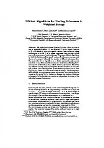
- (2) � b ? (3)
Figure 5.1: Quiver for A51 Problem Instance. with the same origin and terminus). What this implies is that when dealing with admissible orders built with the left lexicographic, how the alphabetic order sequences the out-arcs of each vertex is all that is important (at least to determining the Gr¨ obner basis for a generating set). Similarly, if the admissible order uses the right lexicographic order, all that matters is how the alphabetic order sequences the in-arcs of each arc. To test this hypothesis, a simple problem instance was chosen and run for all possible permutations of the arcs. The graph for this instance is shown in Figure 5.1. The graph has six arcs and so 720 possible alphabetic orderings (modulo the ordering on vertices). Two orders were used for the test: the length lexicographic order, and a weight order that makes da < e. The results divided into four classes depending on the relationship between d and e and the relationship between a and c. Table 5.10 shows the results for each class (all numbers were the same for all alphabetic orders in each class, and every instance resulted in a finite Gr¨ obner basis). The hypothesis would suggest that the relationship between d and e would be significant, but the relationship between a and c is unexpected. One explanation of the importance of the order between a and c is that it is significant to the selection strategy for this particular problem. If this is true, it would mostly explain why the alphabetic order has such a strong influence on the computation. That is, since the selection strategy appears to have the most significant impact on the time required for the computation, the alphabetic order determines which common multiple is chosen (among those of the same length). Further experiments are needed to test how the alphabetic order influences selection and the rest of the computation.
Benjamin J. Keller
Chapter 5
90
Table 5.10: Counts for Classes of Alphabetic Orders on Problem A51. Constraints
Order
d > e, a > c
Length Weight Length Weight Length Weight Length Weight
e > d, a > c d > e, c > a e > d, c > a
5.7
% Nonzero Reductions 79.41 92.50 78.94 90 80.30 89.78 83.33 91.30
Maximum Overlaps 848 1729 380 1598 3100 8707 516 2229
Maximum Cardinality 163 256 54 127 369 691 66 322
Summary and Directions
In Section 5.5 a ranking of seven orders considered is given. This ranking indicates that the first order to try is the length order. In fact, this is what string rewriting folklore and our experience over the course of this research suggests. However, the ranking is not really valid because the experimental results do not imply a total ordering of the admissible orders. In fact, the results seem to imply that which admissible order is best for a particular problem really depends on the alphabetic order. Although some experiments with alphabetic orders have been done, there is no obvious result that indicates how to choose the best alphabetic order. In fact, the results in the previous section can be interpreted as showing the influence of the alphabetic order over the selection strategy. Perhaps using an implementation that allows the use of different alphabetic orders for the selection strategy and the polynomial order would be helpful in experiments to understand the choice of alphabetic order. Another approach that might be more practical than a simple ranking of orders, is to develop heuristics for choosing an order for a particular problem. If we reconsider the criterion for ranking the orders defined in the previous section, the best orders for a generating set P are those for which P is a Gr¨obner basis. This means that either there are no overlap relations for P , or they all reduce to zero. In general, the criterion translates to the best order being the one for which there are the least number of overlap relations throughout the computation. A heuristic based on this idea is to find an order that minimizes the number of overlaps of the generators. Refinements of this heuristic might try to minimize overlaps that would occur in later stages of the algorithm.
Benjamin J. Keller
Chapter 5
91
An approach of this sort might prove to be more practical, and certainly simpler to find than a characterization of which orders are the best for which problems. The following chapter explores the relationship between orders and problems in path algebras as an alternative approach to the problem of choosing an order.
Chapter 6
Admissible Orders in Path Algebras This chapter explores the relationship between admissible orders and problem instances. The experiments in Chapter 5 suggest that the choice of order is highly dependent on the problem instance. For free algebras, the problem instance is determined by the relations, but in path algebras with more complex quivers, the quiver determines what words appear and so also affects the choice of order. This chapter explores the relationship between a graph and the orders on its paths. While the experiments in Chapter 5 also indicated that the relations have more of an effect on the choice of order, this relationship is not considered here. In particular, this chapter looks at equivalence classes of orders on paths induced by the structure of the corresponding graph. The goal is to identify representatives of equivalences classes of orders. The equivalence we consider is whether two orders induce the same Gr¨obner basis (or at least the same tip set) for a given generating set and is defined in Section 6.1. Section 6.2 begins the development of an approach to the computation of representative orders for the equivalence classes for very special graphs. This approach uses a relationship of spanning trees and admissible orders observed by Green [24]. Once this approach is complete, it might be possible to combine it with an approach using information on the generating relations to make the choice of order. This and other future research directions are discussed in Section 6.3. The work by Martin [41] on determining orders that induce termination of string rewriting
92
Benjamin J. Keller
Chapter 6
93
systems is related and could be useful. The result on spanning trees given below is an observation of Green.
6.1
Equivalence of Orders
Two orders are considered to be equivalent for a particular problem instance if the resulting Gr¨ obner bases are the same. Theorem 6.1 given below says that it is sufficient to consider only how two orders sequence the uniform equivalence classes. First we define some notation. Fix a finite directed multigraph Γ = (Γ0 , Γ1 ). Suppose that < u, v ∈ Γ0 are vertices, and < is an admissible order on B the set of paths of Γ. Denote by Eu,v
the ordered sequence of uniform paths between u and v, and (in a slight abuse of notation) let