Tutorial: Supervised Neural Networks in Machine Vision. - Tina

Tina Memo No. 1997-003 Internal.

Tutorial: Supervised Neural Networks in Machine Vision. N. A. Thacker. Last updated 1 / 12 / 1998

Imaging Science and Biomedical Engineering Division, Medical School, University of Manchester, Stopford Building, Oxford Road, Manchester, M13 9PT.

N.A.Thacker

1

Introduction

Neural network architectures can broadly be divided into two classes; • unsupervised algorithms • supervised algorithms The work done in these two areas tends to be motivated by different goals. The unsupervised architectures are generally motivated as models of physiological systems, the main goal being the attainment of self-organisation. This is the process whereby a system automatically learns to extract useful information from input data analogous to the process of cluster analysis in the field of pattern recognition. The most popular network architectures that fall into this category include ART [3] (the early versions of which are almost indistinguishable from the socalled leader clustering algorithm) and the Kohonen net [11]. The ART networks provide a reasonable functional simulation for some parts of the brain based on physiological models but as yet provide very little which is of genuine use for algorithmic research. The Kohonen Net is intrinsically linked to the idea of topographic mapping and provides a useful technique for mapping high dimensional data sets in fewer (typically two) dimensions. Again, however, in terms of algorithmic novelty their performance is almost identical to the nearest neighbour classifier [8] and provide very little additional advantages outside its use as a data visualisation tool. Supervised network algorithms on the other hand tend to be motivated by requirements of a system to perform a specific task. This leads to well defined training algorithms which can be designed to optimise specific statistical performance criteria. These networks can be defined for both ‘static’ and temporal sequence pattern classification though only static pattern classification will be covered here. When considering the application of neural networks to research in machine vision there are several limitations of these algorithms which need to be considered. Feed-forward neural networks are simply a high dimensional interpolation system and can only reproduce one-to-one or many-to-one mappings. As a consequence, use of these methods can give no advantage over standard techniques if there is an accurate model for the system. Where there is no model for the system then neural networks can be expected to work only as well as other non parametric methods. They can only be expected to perform better than parametric methods if the assumptions of the selected parametric model are inadequate. Conventional architectures do not generate meaningful internal representations due to a limitation caused by the initial selection of network architecture. They are therefore not effective at extracting relevant invariant relationships between conjunctions of input features. Traditional neural network architectures are notoriously difficult to train efficiently [25]. The other problem is that the training time required for a particular mapping task grows as approximately the cube of the complexity of the problem. This prohibits the use of standard neural networks on all but the simplest and most straight-forward of tasks. In conclusion, functional mapping networks can currently only be of real value in limited complexity problems where most of the required output mapping (invariance) characteristics have already been built into the input data. Even with this restriction these techniques can be of real use in machine vision. After describing briefly the knearest neighbour classifier the following sections will focus on the aspects of supervised feed-forward architectures including; • network architecture. • statistical optimality criteria. • training algorithms. • statistical testing. • machine vision applications.

2

K-Nearest Neighbour Classification

The K-nearest neighbour classifier is by far the most popular technique for forming classification decisions for cases where a large quantity of training data is available. The technique involves computing the distance of an input

2

vector Ii from a set of stored training examples wij assuming a suitable distance metric is known. This often takes the form of the Euclidean or Mahalanobis distance metrics: X (wij − Ii )2 Ej = i

and the more general Mj = (wj − I)T CI (wj − I) (subscripts have been dropped to imply vector quantities). The distance metric is generally selected for computational convenience and rarely because of statistically valid reasons, although the technique will have statistical validity if the ”covariance matrix” CI is selected to model measurement errors on I. The classification decision is then simply done on the basis of majority voting of classification of the K nearest patterns. The reason for the popularity of this technique (besides simplicity) is that it can be shown to approach Bayes optimal classification performance for large data sets. Bayes optimal is defined as obtaining the error rate we would achieve if we knew the underlying probability distributions which generated the data set and were to use them at each point in the input pattern space in order to make our classification decision. This technique is closely related to the Parzen classification approach, where an attempt is made to estimate the underlying probability distributions more closely, for a more detailed description of this and associated techniques the reader is referred to [8]. For small data sets however, the technique is highly dependent on the selection of the distance metric. Supervised learning approaches to neural network pattern classification have the freedom to learn underlying statistical trends in the data thus eliminating the ad hoc choice of distance metric and enforcing local smoothness constraints in the decision surface which help to cope with small data sets. It must still be said, however, that in the majority of cases a nearest neighbour classifier, by approaching closely Bayes error rates, will be sufficient for a pattern classification problem and application of neural network techniques may be completely unwarranted.

3

Feed-forward Network Architecture

The general network structure (figure 1) and the back-propagation algorithm [21] are now well established in the literature. A vector of input components Ii is fed directly to the output oi of the input layer i of nodes (in CMAC networks and fuzzy systems oi may also be a linear function of I, but this is beyond the scope of this review) and the activity at subsequent nodes is calculated from the equations. X dj = wij .oi i

or rj =

X i

and

(wij − oi )2

oj = f (dj ) or

g(rj )

Where wij is the connection strength of the wire between nodes i and j. Notice the similarity of the r j function to the nearest neighbour algorithm, nearest neighbour classifiers thus form a sub-set of the neural network approaches. The nearest neighbour algorithm is in no way unique in this respect, as neural network approaches can now be shown to contain many standard statistical pattern recognition formulations as a sub-set. The main difference being that parameters are determined by a training process and would probably have been assumed to be known in the statistical approaches. The input function often also has a bias weight term, but this can be accommodated within this mathematical model by connecting a bias node (with fixed output and no inputs ) to node j. The usual choice for the transfer function f (d) for Multi-Layer Perceptrons (MLPs) is the ogive ( or sigmoid ) f (d) =

1 1 + exp(−d)

For Functional Link Nets (FLNs) the choice is f (d) = dn

polynomial

3

t o

k

training data

k

outputs output layer

o = f(I ) j j

hidden units I = j

w ij

or

input layer I

i

w o ij i

I = j

inputs

(

w ij

-

o) i

2

Figure 1: Feedforward Network Architecture f (d) = sin(d) f (d) = cos(d) f (d) = tan(d) Finally for Radial Basis Function (RBF) networks the following selections are typical g(r) = exp(−r 2 /2σ 2 ) g(r) = r2 log(r) 2

2 1/2

g(r) = log(r + σ )

Gaussian thin plate shif ted log

The activity at the output layer is calculated by computing the output from each layer of nodes starting from the input values and working towards the output. There may be several internal layers of nodes before the final output layer. Training proceeds by changing the weight values (set initially to sensible random values) so that the next time each particular pattern is presented the output generated is more like (by some pre-determined metric) the required result. This training procedure can be organised in several ways which will be discussed. Although in principle a single network can be used to estimate multiple outputs there is rarely merit in attempting this. Consequently problems are often broken down so that each required output is estimated from a different network. Very little will be said in this review about the choice of particular architectures for specific problems. This is because, on the whole, most of these networks will estimate an arbitrary functional mapping as well as another given an equivalent number of free parameters. This assumption does have a few key exceptions. Firstly when performing classification tasks MLP architectures tend to be more compact than their RBF counterparts (often by an order of magnitude) as it is more efficient to describe decision boundaries through a space than to map each distinguishable point. RBF networks on the other hand tend to be better at general function interpolation and can also be designed to indicate if the input pattern is within the known domain of the original training data. Finally RBF networks can tend to have better interpolation performance if the outputs from the intermediate (hidden) nodes are positive and normalised, as this forces the network to interpolate between limits set by the maximum contribution of the weights connecting to the output layer. Specific choice of neural architecture can also impose a direct probablistic interpretation on internal network function [19] as well as just the training algorithm, as will now be describe below.

4

Statistical Optimality Criteria

One of the most important results to emerge from the neural network literature in recent years is that under certain conditions they can be shown to estimate Bayesian conditional probabilities. These conditions involve selection of a particular training regime and a complementary optimisation function. For example, the most common optimisation function is the least squares error criteria which summed over the entire data set for output k gives X Ek = (o(In ) − tnk )2 n

4

where tnk is the nth training output and o is the output from the network for a particular input In . The obvious interpretation for this training algorithm is that our training outputs are Gaussian distributed random variables. However, we can also show that there is another link with probability theory which is broader in scope and therefore much more powerful. Provided that we are training with data which defines a 1-from-K coding of the output (ie classification) we can partition the error measure across the K classes according to their relative conditional probabilities p(C k |I) so that XX Ek = (o(In ) − tnk )2 p(Ck |In ) n

k

expanding the brackets Ek =

X n

=

(o2 (In ) − 2o(In )

X n

X k

tnk p(Ck |In ) +

X k

t2n p(Ck |In ))

(o2 (In ) − 2o(In ) < tk |In > + < t2k |In >)

where < a|I > is the expectation operator of a at In . By completing the square this can now be re-written as X X var(tk |In ) (o(In )− < tn |In >)2 + Ek = n

n

The last term is purely data dependent so that the only effect that training can have is to minimise the first term which is clearly a minimum when o(In ) = < tk |In >. For a 1-from-K coding of the output and in the limit of an infinite number of samples < tk |In > = P (Ck |In ). Thus under these conditions neural networks trained with the least squares error function will approximate conditional probabilities of classification. Notice that the error function itself E is not necessarily defined as an expectation value (as it is in [19]) and the output will estimate conditional probabilities provided that the ratio of output samples necessary to define < t k |In > at each point In in the data set is preserved. This suggests that in many problems a set of training data can be ‘thinned’ by a clustering process and the data at each distinguishable input position averaged, in order to reduce network training time, without loss of this useful interpretation of data output. Another cost function often defined for network optimisation is the cross-entropy function X Ek = − tnk log(o(In )) + (1 − tnk )log(1 − o(In )) n

This is motivated by the assumption that desired outputs tnk are independent, binary, random variables and the required output network response represents the conditional probability that these variables would be one. The proof of this follows as above with the introduction of the partion of the classification state over the one and zero cases eventually giving X Ek = − < tk |In > log(o(In )) + (1− < tk |In >)log(1 − o(In )) n

which when differentiated with respect to the desired output shows that this function is minimised again when o(In ) = < tk |In >. Again for 1-from-K classification problems these conditional expectations are the Bayesian probabilities. In practical circumstances there has been very little evidence to show that either of these measures (least-squares or cross-entropy) result in significantly better performance than the other, though it is interesting to note that theoretically there are strictly defined domains for correct application. What is important from the algorithmic point of view is that once we have shown how neural networks can approximate conditional probabilities they are no longer black boxes with ill defined magical properties. In particular neural networks can only achieve Bayes optimal classification and estimation behaviour and therefore cannot out-perform the appropriate standard methods if one is applicable. As will be shown later however, there are some applications where direct estimation of conditional probabilities represents a useful step forward in algorithmic practice.

5

Training

For many network architectures once the cost function has been specified the training of the network can be accomplished by treating the problem as one of standard parameter estimation. Many networks (particularly RBFs) 5

can even be trained by making use of psuedo inverse techniques [5] (commonly singular valued decomposition). However such techniques are generally unwieldy for large networks and iterative techniques, requiring less data storage, are preferred. These techniques are even applicable to problems in adaptive control and the extended Kalman filter can be used to update the weights in an optimal (least-squares) manner. For the remainder of this report we will concentrate on the standard back-propagation algorithm and extensions which lead eventually to the standard conjugate gradient schemes. None of these minimisation techniques are particularly specific to a particular network architecture or optimisation function and the basic approach can be used to develop learning algorithms for any feed-forward network. Back-propagation is a training algorithm used to make a layered network learn a functional mapping between a set of input patterns and their respective outputs. The networks take the form of a set of input units connected by wires to an arbitrary number of hidden units, which are connected in turn to output units. It is assumed that each unit in the network is a simple processing element. These produce an output which is simply a differentiable function of the sum of the weighted inputs from the nodes to which it is connected. In principle any unique mapping can be learned, in practice however there are several numerical problems which have to be addressed first. The first problem is that the original gradient descent method (and its modifications) have a number of free parameters which affect the convergence of particular networks differently. The best parameter values for a given network mapping cannot be predicted in advance and slight misjudgement in the choice of these parameters can cause problems with convergence. Also, no methods yet exist for predicting the optimal network architecture for a given mapping problem. These two factors make the application of such networks to even the simplest problem difficult, because if a particular network does not converge we may not know which is responsible. Also, there is no guarantee that choice of the correct parameters and architectures will generate a particular mapping. This is because the back-propagation algorithm is a minimisation algorithm which is subject to the same local minima difficulties as any other such method. Network modules are likely to grow larger as the problems they are used to solve become more complicated. It has thus been considered important to try to improve the training algorithms and see if any better methods can be found which have fewer unknown factors and are less sensitive to the starting conditions in the untrained network (ie robust). We may then be able to develop systematic methods for the application of these networks to specific classes of problems.

6

Back-propagation by Gradient Descent

The training of the network can be envisaged as the minimisation of an error function E n X En = (ok − tnk )2 k

where tnk is the required output from node k for input pattern n. This (least square error) is the best quantity to use if the training data is expected to have uniform Gaussian errors and also for the reasons mentioned in the previous section. This equation allows the calculation of the quantity ∂En /∂wij by repeated application of the chain rule. ∂En /∂wij = ∂oj /∂wij .∂En /∂oj X ∂En /∂oj = ∂En /∂wjk .wkj /oj k

For the sigmoid transfer function given earlier this derivative calculation is of a particularly simple form. Most of the computation necessary is done during the forward pass so that we almost get the derivative information free [15]. Calculation is done starting from the output layer and working backwards towards the input layer hence the name back-propagation. Training can then be achieved by changing all of the weights in the network by a small amount in this direction. ∆wijn = α∂En /∂wij Where α is known as the learning rate and simply determines how far each minimisation step attempts to move in the downward direction. At first this appears a sensible training strategy as the data can be presented in any order and there is only one free parameter α. However, this one free parameter is not easy to choose as too small a value will result in a long convergence time and too large a value will result in unstable learning. Further the optimal value will vary during minimisation thus the method cannot be expected to reach the minimum in all cases. Worse still is the fact that 6

there is no effective way of monitoring the overall learning state of the network. Although the network will improve its ability to reproduce each particular output at each step there is no reason to expect that this improvement will not be undone by some future learning step. In fact as a minimisation method this is almost certainly the slowest and least robust of all. Some of these problems are however solvable as will be shown below.

7

Back-propagation with Momentum Terms

The first thing to do is to adopt the method generally referred to as batch training and define the error function so that it encompasses all of the available data. Then the total error function is simply redefined as X E(τ ) = En n

with ∂E(τ )/∂wi j =

X

∂En /∂wij

n

Now we can use this quantity after each epoch τ of training (one epoch defined over the whole data set) as a measure of the success of the training. Also we can modify the learning algorithm to include an extra term ∆wij (τ ) = α∂E(τ )/∂wij + η∆wij (τ − 1) η is generally called the momentum term and does two things. First it smooths out local irregularities in the minimisation function allowing the gradient descent to follow a consistent path. Secondly it allows the minimisation process to increase in speed when there are long periods of identical gradient evaluations. These properties make this method an order of magnitude more efficient than the previous. Despite these improvements, it is this “Vanilla” form of the back-propagation algorithm, with two unknown free parameters, which is unreliable and requires much effort to obtain repeatable minimisation for a particular problem. Yet it is this form of back-propagation which is the base learning algorithm for much research.

8

RPROP.

RPROP is an acronym for “Resilient Back-Propagation” and is a locally adaptive learning scheme which aims to improve the robustness and speed of the “Vanilla” scheme. The technique is based on the assumption that there will be some instability in the gradient estimation process which will lead to oscillatory effects during network performance optimisation. The training regime attempts to overcome this problem by removing the harmful influence of the size of partial derivatives in order to stabilise the weight modification process. As a consequence only the sign of the derivative is considered to indicate the direction of the weight update. The size of the weight change is exclusively determined by an update value ∆ij (τ ) according to ∆wij (τ ) = − ∆ij (τ ) , if ∂E(τ )/∂wij

> const

∆wij (τ ) = + ∆ij (τ ) , if ∂E(τ )/∂wij

< const

∆wij (τ ) = 0 , else where const is determined according to machine precision and the update values are computed according to, ∆ij (τ ) = η + ∆ij (τ − 1) , if ∂E(τ − 1)/∂wij ∂E(τ )/∂wij

> const

∆ij (τ ) = η − ∆ij (τ − 1) , if ∂E(τ − 1)/∂wij ∂E(τ )/∂wij

< const

∆ij (τ ) = 0 , else Where η + and η − are predefined constants. This algorithm has been shown empirically to have good convergence properties, particularly for problems which have irregular error minimisation surfaces (ie those which are not well approximated by a quadratic). Full details can be found in [20]. 7

9

Back-propagation with a Simple Feedback Loop

In order to understand the problem of network training stability it is instructive to automate the selection of learning rate using feedback information. Before we do this it is best to reformulate the calculation of the weight change. vij (τ ) = ∂E(τ )/∂wij + βvij (τ − 1) ∆wij (τ ) = αvij β must be chosen in the range 0-0.5 if the previous direction calculations are not to have greater significance than the current derivative in the calculation of the new minimisation direction vij (τ ). This value is thus easier to specify than the η term and a value of 0.3 is normally used. These changes give α better control of the learning rate and make the new term β responsible solely for smoothing the direction of descent. Also, It should be noted that this formulation is directly comparable to that of the conjugate gradient method which will be described later. Using the derivative information we can explicitly compute the expected reduction in the error function by propagation. X ∆wij (τ )∂E(τ )/∂wij . ∆Ee (τ ) = ij

Where the summation subscript ij implies all wires in the network. This can then be compared with the achieved value, if they are almost equal (within a few percent) then the linear prediction from the gradient is accurate so we must be on a downward slope relatively free from second order terms and we can therefore increase α with safety. If however the prediction does not agree with the results we must proceed more cautiously and the learning rate must be reduced. The required rate of change of the learning rate is a direct measure of the stability of the training process. An algorithm of this type has been found to be significantly faster than the previous methods and also more stable. The method is not entirely robust as occasionally the feedback mechanism cannot respond quickly enough to local changes in the gradient of the error function. This can however be remedied by storing the last successfully computed point and this is a generally useful strategy for all training algorithms. Other researchers have implemented feedback modifications based on the achieved minimisation at each step [25]. These can be implemented as simple extensions to the original algorithms and result in a similar increase in minimisation speed.

10

Back-propagation Using Conjugate Gradient Descent Methods

In order to remove the final free parameter from the minimisation process we must find some way of determining the optimal value for β locally. In fact an existing minimisation method, known as conjugate gradient descent, does just this and in a way that can be shown to produce an efficient search for the minimum. The algorithm assumes that we wish to take steps in an approximate downhill direction vij (τ ) (as above) such that each step is always conjugate to any of the previous steps. This removes the oscillatory behaviour of pure gradient descent methods and is super-linearly convergent (ie fast) in the region of a quadratic minimum. It can be shown that such directions can be constructed iteratively from the error derivative provided that each derivative evaluation is done at the minimum along the direction of the previous conjugate direction (for details see Numerical Recipes in C. 1988) with P ij (∂E(τ )/∂wij − ∂E(τ − 1)/∂wi j).∂E(τ )/∂wij P β(τ ) = ij ∂E(τ − 1)/∂wij .∂E(τ − 1)/∂wij

As successive derivative directions are generally orthogonal, this is no more than the square of the magnitude of the new derivative divided by the square of the old. This is the Polak-Ribiere implementation of the algorithm which allows the direction to revert to the downhill direction when in difficulty. Implementation requires a method of finding the α(t) which gives the minimum of the error function in this direction and in doing so also determines its optimal value for each step. This linear search for the minimum has to be done in two stages, first the minimum must be bracketed and then the position of the minimum needs to be determined to a specified accuracy within this bracket. One method for bracketing the minimum is a down hill step search, combined with parabolic extrapolation once three or more evaluations have been done. The minimum can then be located using a golden section search algorithm [18], one of the simplest and most robust methods for this task (given that the error function is not likely to be well

8

behaved). The number of function evaluations in each line minimisation can be regulated using the required fractional minimisation at each step without any loss of robustness. This algorithm is the most stable of all the iterative methods mentioned so far, though RPROP has been found to cope better with multiple minima. It has essentially no free parameters as they are all either determined at each step or specified by the floating point accuracy of the implementation. However, the efficient search through the minimisation space is offset by the increased number of function evaluations so that the overall minimisation time is approximately the same as for the methods with feedback. Also, its very robustness now heightens the problems associated with encountering local minima which have to be addressed.

11

Problems with Local Minima

Knowledge of the expected errors on the training data should be used to determine a sensible value for the desired error function and once below this there can be little point in attempting to leave local minima. Indeed continuing minimisation may be entirely the wrong thing to attempt as any local minimum may embody a logically viable solution. However, if considerable computing time has been invested in training and a local minimum is found, such that the value of the error function is not satisfactory, then it would make sense to try to find a way out of the local minimum so that learning can continue, rather than having to restart the training from a different (probably random) position. The conjugate gradient minimisation algorithm described above is extremely robust and can be implemented in such a way that it never fails to find a minimum. However, there is no guarantee that the minimum found will be the ‘true’ global minimum or even close to this. The less robust gradient descent methods can sometimes ‘tunnel’ out of these minima, but the conjugate gradient descent method will be stuck. Much work has already been done on this general minimisation problem but in the case of network training with a least-squares cost function there is a method available which requires only a slight modification of the existing algorithm. Ignoring for the moment the statistical interpretation of the error function, the choice of norm is in most respects arbitrary. In fact we can choose any continuous difference metric we like, to quantify the difference between the obtained and the required output. Specifically we can use any metric of the form E(τ ) =

X

h(

n

X k

g(ok − tnk ))

which will force ok = tnk after training. We can expect different forms of this error function to have different local minima in many cases and we will generally expect only the global minimum to be reproducibly coincident. We can use this as a basis for a controlled method of walking out of local minima. When a local minimum is encountered the value of the error function is stored and a different error function is used until the evaluation of the old function is less than the stored value. By definition the new position must be outside the region of the previous local minimum and we can revert to the original error function in order to regain a statistical interpretation for the performance of the trained network. The preferred error function for this purpose is E 0 (τ ) =

XX ( (ok − tnk )2 )2 n

k

as this leads to a simple extension to the existing derivative calculation XX ∂E 0 (τ )/∂wij = (ok − tnk )2 ∂E(τ )n /∂wij n

k

This was motivated by the observation that local minima were often the result of a few badly learned mappings and places emphasis on their contribution to the error function and its derivative. In most minimisation problems encountered this method has been found sufficient to escape local minima, allowing minimisation to continue using the original error function.

12

Statistical Testing

The final problem encountered in the application of neural networks to a practical problem is in understanding network performance. This process is fundamental to the problem of trying to select an optimal architecture for 9

the mapping task. The final cost function value after the training process provides only a best case estimate of performance. Further, increasing the complexity of the network will always improve the ability of the network to map the training data though this may reduce the ability of the network to provide accurate outputs for unseen data. This problem is generally referred to as the bias-variance dilemma [9]. In order to check that a particular trained network will ‘generalise’ to unseen data, it is common to withhold some proportion of the data from training and then test with this data. For small quantities of initial training data this can lead to the problem of having insufficient data for either training or effective testing. The common solution to this problem is known as ‘jack-knifing’ or the ‘leave-one-out’ strategy. One data point is omitted from the data set and a network trained on the rest. The performance of the network is then tested on the remaining point. This process is then repeated with the same architecture initialised with different random weights, each time removing a different data point. By this process we eventually build up a statistical estimate for the generalisation capabilities of a particular architecture type which can be compared across several architectures to determine the best one. Recently it has been suggested that it may be possible to estimate the performance of a network by using what is effectively a Bayesian stability analysis with the original data [17]. If this method is correct then it provides a way of estimating the generalisation abilities of a specific network (and weights) while also allowing training on the complete data set. In some cases we wish to use a network to map an output from an ordered sequence of values, such as temporal measures. In this case it is possible to use a wide range of correlation measures to verify the adequacy of the mapping [4]. Strong correlations between points of fixed separation in time will indicate a functional bias.

13 13.1

Machine Vision Applications Feature Detection

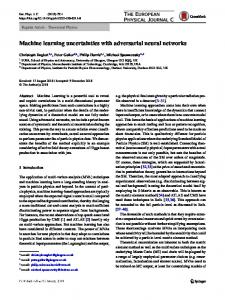
As mentioned above, neural networks can be useful in machine vision in circumstances where conventional methods do not provide outputs which are well related to conditional probabilities. One example of such a process is feature extraction, such as edge or corner detection where a network can be taught the mapping from a region of image pixels to an output central pixel label. Conventional detectors are often based on ideas of image calculus and deliver results which can be systematically wrong (in terms of a strict definition of a real 3D feature) and unreliable. One possible barrier to using neural networks is that the scale of the learning problem is vast for reasonable sized input image patches. In order to reduce the scale of the required mapping it is sensible to perform image normalisation before inputting the data to the network (figure 2). Each factor γ of unnecessary data variation which is removed will reduce the overall size of the network required to learn the problem by the same factor and will reduce the total learning time by as much as γ 3 . By training a neural network to extract features from images we get several benefits. Firstly if we can correct systematic effects in the detection algorithm during generation of training data, the neural network will learn to extract the feature without bias. Secondly the neural network can be made to deliver conditional probabilities for the detection process so that we will know not only where a feature is but how likely it is to be recovered in subsequent frames of the same scene. Thirdly, the network training process can explicitly take into account effects of quantization and the actual active area of the image pixel sensors. Finally, neural networks provide a common computation framework allowing the construction of compact general purpose feature detection hardware.

13.2

Object Location

A technique which has received much attention in the literature in recent years is point distribution modelling. This technique can be used in a supervised training regime to learn the allowable variations in shape and grey-level values for a set of image data. These constraints can then be used in a relatively efficient manner in the process of object location. The simplest correlations between position and grey level variation are based on standard statistical assumptions of linear independence and Gaussian distributed data. However, for some objects these correlations may be distinctly non-linear and such techniques are inadequate and can result in poor performance during object location. In such cases a neural network can be used to generate an alternative representation of the input data such that linear independence can be assumed [22].

10

Key:

x

I - Input image region.

G

∆

log - Logarithm.

|

∆

log

|

∆

I

2

DR

NN

O

- Gradient.

G - Gaussian Convolution. - Patch Rotation.

y

DR - Dimensional Reduction.

G

NN - Network Classifier.

∆

O - Bayes Probability Output. Figure 1. Data flow in the Invariance Network Architecture.

Figure 2: Invariance Network Architecture

13.3

Data Fusion

A problem that arises frequently in machine vision is that of data fusion, how to combine data from separate decision/classification systems. Often if the output of two modules can be interpreted as conditional probabilities, we may be tempted to multiply the outputs of two systems in order to get an overall result p(Cm |A, B) = p(Cm |A)p(Cm |B) Strictly this combination process is only correct for uncorrelated events. As a neural network estimates Bayesian probabilities we may instead choose to train a network to estimate a combined response from two classifiers. However, in this case the network will not estimate p(Cm |A, B) but instead p(Cm |p(Cm |A), p(Cm |B)). If we are in the process of constructing a hierarchical classification system and want to work with partial data sets to form intermediate probabilities this is a sensible way to solve the problem. In addition if the vector of output classifications p(C|X) allows us to uniquely specify the original input data X for each X then p(Cm |p(Cm |A), p(Cm |B)) = p(Cm |A, B) as no information is lost due to the initial classification processes. For sufficiently rich classification classes we may expect this condition to be approximately true. This data combination process has been applied to the problem of texture classification and segmentation [1].

13.4

Object Recognition

The problem of general purpose object recognition has long vexed the machine vision community. The mindless application of the networks described here would not be expected to be fruitful for this task because of the scale of the learning problem. However, Wechsler has demonstrated [26] that by applying suitable pre-processing schemes (figure 3) to image regions some useful recognition abilities can be learned.

13.5

Robot Control

Another use of these networks is in solving the inverse kinematic problem [6]. This is the problem of finding the optimal way of converting from normal cartesian co-ordinates into the configuration space of robot joint angles. The forward calculation from joints to space is trivial, given an adequate model of the robot, but the inverse kinematic problem was definitely not. However, it is such mappings as these that neural networks learn with ease. Many examples of the forward kinematics and the resulting robot arm position are used as training examples for the network. This process is often referred to as inverse system identification. Once trained these networks provide quicker solutions than the conventional computational approaches. This elegant solution suggests many potential applications of networks to inverse mapping problems, for instance “shape from ” modules [12]. Hence, feed-forward networks must be considered as a useful tool for solving many computational problems.

11

2D Object Recognition (Wechsler 1989). 512x512 8bit image

Centroid Location (Corner Detection) Log-Polar Mapping 64x64 pixels 14 bit Edge Enhancement. (Laplacian) 64x64 pixels 16 bit 2D Fourier. 64x64 pixels 16 bit Neural Network (MLP)

Object Classification Likelihoods Figure 3: Object Recognition

14

Software

Finally, on the subject of neural network research, it remains for me to point out that a considerable quantity of software has been written in both the industrial and academic sector for the application of neural networks. It therefore makes sense to try to make use of such software in future work, rather than have to reimplement everything that has been done before by many other people before the process of application research can commence. In many cases it is sensible to visualise the data, particularly before attempting neural network classification. As if the data is trivially separable, neural network approaches may be unwarranted. The package XGOBI, available as free software from CMU is ideal for this task. For the purpose of network generation and training I would recommend the Stuttgart Neural Network Simulator (SNNS) [27] which is available as free software from the University of Stuttgart. This software is easy to use and well documented, with complete descriptions of the various training algorithms and architectures. Finally, in order to manipulate images to generate data for training I would recommend our own TINA vision system [24] (available as free software from the University of Manchester) which comes complete with many standard vision algorithms and interfaces easily with these other two packages on UNIX platforms.

15

Conclusion

A brief overview of the design of neural networks and their potential for use in machine vision applications has been given. A more complete description of individual network algorithms can be found in [14] with a more up to date review in the follow up paper [10]. There are also some very good textbooks available [2, 26]. The fundamental aim of AI research must be to develop systems which are capable of learning so that they are not limited to the knowledge available at the time of construction. Such systems may then be capable of extending 12

their knowledge and eventually exhibiting truly intelligent behaviour. In this respect neural network research is currently one of the few fields which may be able to support artificial intelligence. However, if neural networks are to provide a full solution, some key issues still need to be answered. Flexible architectures need to be developed which can cope with the problems of noisy data and can efficiently combine multiple sources of information. Architectures such as this have been suggested in the literature but are highly specialised and beyond the scope of this general review [23]. Integration of the temporal dimension into network function will also be important for a large class of applications [16]. Algorithms need to be developed which train and modify these networks automatically in a robust manner [13], or at least allow a working definition of efficiency by which to optimise the network architecture for a given problem.

References [1] D.Booth, N.A.Thacker, M.K.Pidock and J.E.W.Mayhew. ‘Combining the Opinions of Several Early Vision Modules Using a Multi-Layered Perceptron.’ Int.Journal of Neural Networks,2,2/3/4,June-December,7579,1991. [2] M.Brown, C.Harris. Neurofuzzy Adaptive Modelling and Control, Prentice Hall, London, 1994. [3] G.A.Carpenter, S.Grossberg,D.D.Rosen. ART 2: ART-2A: An Adaptive Resonance Algorithm for Rapid Category Learning and Recognition, Neural Networks, Vol.4, No.4, pp. 493-504. 1991. [4] S.Billings and W.Voon, Structure Detection and Model Validity Tests in Identification of Non-Linear Systems. Proc. IEE. Part D, Vol 130, 193-199,1983. [5] D.S.Broomhead, D.Lowe, Multivariable Functional Interpolation and Adaptive Networks, Complex Systems, Vol 2, pp. 321-355, 1988. [6] R.K. Elsey, A Learning Architecture for Control Based on Back-Propagation Neural Networks. Rockwell International Science Center 1988. [7] A.C.Evans, N.A.Thacker and J.E.W.Mayhew, The Use of Geometric Histograms for Model-Based Object Recognition, Proc. 4th BMVC93, Guildford, 21-23 pp429-438 Sept. 1993b [8] K.Fukunaga. Introduction to Statistical Pattern Recognition, 2nd Edition, Academic Press, London. 1990. [9] S.Geman, E.Bienenstock, R.Doursat. Neural Networks and the Bias Variance Dilemma, Neural Computation, Vol4. No1, pp 1-58. 1992. [10] D.R.Hush,B.G.Horne. Progress in Supervised Neural Networks: Whats New Since Lippmann?, IEEE Sig. Proc. Mag., pp 8-39, Jan 1993. [11] T.Kohonen. The Self Organising Map, proc. IEEE, Vol. 78, No.9, pp 1464-1480. 1990 [12] S.R.Lehky T.J.Sejnowski, Network model of shape from shading: neural function Arises from both receptive and projective fields. Nature Vol 333,452-454 June 1988. [13] R. Linsker, Self-Organisation in a Perceptual Network. IEEE Computer 105-118 March 1988. [14] R.P.Lippman, An Introduction to Computing with Neural Nets. IEEE ASSP Magasine April 1987. [15] J.L. McClelland D.E. Rumelhart, Parallel Distributed Processing. MIT press Vol 1 322-328 1986. [16] N. McCulloch, Methods of Incorporating Time into Artificial Neural Networks. RIPRREF /1000 /30 1988. [17] D.J.C.Mackay., Bayesian Modelling and Neural Networks, Research Fellowship Dissertation, Trinity College, Cambridge, 1991. [18] W.H.Press B.P.Flannery S.A.Teukolsky W.T.Vetterling Numerical Recipes in C. Cambridge University Press 1988. [19] M.D.Richard,R.P.Lippman. Neural Network Classifiers Estimate Bayesian a posteriori Probabilities, Neural Computation, 3, 461-483, 1991. [20] M. Riedmiller and H. Braun. A Direct Adaptive Method for Faster Back-Propagation Learning: The RPROP Algorithm. Proc. IEEE. Conf. NN 1993. 13

[21] D.E. Rumelhart G.E. Hinton R.J. Williams, Learning Representations by Back-propagating errors. Nature 323,533-538,1986. [22] P.E.Sozou, T.F.Cootes, C.J.Taylor and E.C.Di Mauro, Non-Linear Point Distribution Modelling using a Multi-Layer Perceptron. Proc. BMVC 95, Birmingham,107-116, 1995. [23] N.A.Thacker, J.E.W.Mayhew, ‘Designing a Network for Context Sensitive Pattern Classification.’ Neural Networks 3,3, 291-299, 1990. [24] ’TINA Programmers Guide’, edited by N.A.Thacker, University of Sheffield, 1996. [25] T.P.Vogl J.K.Mangis A.K.Rigler W.T.Zink D.L.Alkon Accelerating the Convergence of the Backpropagation Method. Biol. Cybern. 59,257-263,1988. [26] Wechsler H. Computational Vision. Academic Press, London, 1990. [27] A. Zell, et al. ”SNNS: Stuttgart Neural Network Simulator”,User Manual, Version 4.0, 1995.

14