after the shape in the 2D image of the 3D shape has be established. .... R is a 3x3 rotation matrix and T is a 3x1 translation vector. о ... image plane and the 3D points a and a′ whose images are A and A' coincide with G (it follows that both A.
A computational model that can recover an object’s three-dimensional shape from only one of its two-dimensional retinal representations Yunfeng Li, Zygmunt Pizlo and Robert M. Steinman Department of Psychological Sciences, Purdue University, West Lafayette, IN 47907-2081, U.S.A. Figure-ground organization must be given to the model because it has no provisions for establishing figure-ground organization on its own. This means that the model can only come into play after the shape in the 2D image of the 3D shape has be established. To do this, the model is provided with information about which: (i) points form edges in the image, (ii) edges and vertices form contours of faces “out there”, (iii) edges and vertices are symmetric edges and vertices “out there”, and (iv) edges and vertices define volume of the 3D object “out there” (this last requirement is less critical because once points and edges are represented in the 3D space, their convex hull defines volume uniquely). This information must be provided because the a priori constraints used by the model constrain shape. We call our constraints: “symmetry, planarity, maximum compactness and minimum surface.” In our usage, symmetry refers to the mirror-symmetry of the object, planarity refers to the planarity of the contours of the object. The compactness of the object is defined as V2/S3 where V is the object’s volume and S is the object’s surface area. The minimum surface of the object is defined as the minimum of the total surface area. It is important to realize that no depth cues, not even binocular disparity, are used to recover the 3D shape of an object from its 2D retinal representation in our model. Depth is superfluous to its operation. Our maximum compactness and minimum surface constraints are completely novel in the sense that they have never been used in a model designed to recover 3D shape. Symmetry and planarity constraints had been used in models that recover 3D shape before. Maximizing compactness is equivalent to maximizing the volume of an object, but keeping its surface area constant. It is also equivalent to minimizing surface area, but keeping the object’s volume constant. Note that the minimum surface constraint is equivalent to minimizing the object’s thickness. The bottom line is that our model recovers the 3D shape of an object from its 2D retinal shape by selecting a 3D shape that is as compact and, also as thin, as possible, from the infinitely large family of 3D symmetrical shapes that have planar contours consistent with the 2D retinal shape used to recover the 3D object. Another way of saying this is that our recovery of the object’s 3D shape reflects a compromise between our novel maximum compactness and minimum surface constraints. The reader should realize that our model belongs to the class of regularization models designed to solve inverse problems (Poggio et al., 1985).
Details of our Mathematics and Computations Applying mirror symmetry and planarity of contours constraints to recover a 3D shape Let the X-axis of the 3D coordinate system be horizontal and orthogonal to the camera’s (or eye’s) visual axis, the Y-axis be vertical, and the Z-axis coincide with the visual axis. Let the XY plane be the image. Let the set of all possible 3D shapes consistent with a given 2D orthographic retinal image be expressed as follows: Θ I = { p(O) = I } ,
(1)
where O and I represent the 3D shape and the 2D image, respectively, and p represents an orthographic projection from the 3D shape to the 2D image. 1 There are infinitely many 3D shapes (O) that can produce 1
Orthographic images are used here because perspective distortions are often quite weak, especially when the objects are not very large and not very close to the observer. The recovery problem is more constrained, and thus, easier when perspective images of symmetrical shapes are used because a single perspective image leads to a unique recovery of shape (e.g., Rothwell, 1995). Note, however, that even with perspective images, constraints will still be needed because recovery is likely to be unstable if visual noise is present.
1
the same 2D image (I) because translating any point on the surface of a 3D shape along the z axis does not change its 2D orthographic image. Consider a subset of ΘI, in which all 3D shapes are mirror symmetric and their contours are planar: Θ I ' = {O ∈ Θ I : O is symmetric and its contours are planar} .
(2)
The following, which is based on Vetter & Poggio (2002), will be used to show how symmetry may be used to restrict the family of 3D interpretations of a given 2D image. Note, however, that this restriction, in itself, cannot produce a unique 3D shape. Additional constraints will be needed to recover a unique 3D shape. Given a 2D orthographic image Preal of a transparent mirror-symmetric 3D shape, and assuming that the correspondences of symmetric points of the 3D shape are known, Vetter & Poggio showed how to compute a virtual image Pvirtual of the shape: Pvirtual = D ⋅ Preal ,
⎡0 ⎢0 D=⎢ ⎢ −1 ⎢ ⎣0
(3)
0 −1 0 ⎤ 0 0 1 ⎥⎥ . 0 0 0⎥ ⎥ 1 0 0⎦
Under this transformation, for any symmetric pair of points Preal = [XL YL XR YR]T in the 2D real (given) image, their corresponding pair of points in the 2D virtual image is Pvirtual = [−XR YR −XL YL]T. The virtual image is another orthographic image that could be produced by the same 3D shape from another viewing direction. Figure 1 shows an example of a 2D real and virtual image of a symmetric wire (transparent) shape. The virtual image is usually different from the real image. This is not true in degenerate cases, where 2D real image is itself mirror symmetric. The 2D virtual and the real images are identical for a symmetric 2D image (up to a 2D translation) which means that Vetter & Poggio’s method cannot be applied. Note also that the 2D virtual image is computed directly from the 2D real image. Knowledge about the 3D shape, itself, is not required. This important fact means that the initial problem of recovering a 3D shape of an object from a single 2D image is transformed into a problem of recovering a 3D shape from two 2D images, one real and the other virtual. Clearly, having two images will lead to having a more restricted family of 3D recovered shapes. This is the main idea behind Vetter & Poggio’s method. We will explain next how the 3D shape recovery problem can be formulated and solved.
Figure 1. The real (left) and virtual (right) images of a 3D symmetric shape. A, B are images of a symmetric pair of points a, b in the 3D shape. A′ and B′ are the corresponding points in the virtual image. Note that when the virtual image was produced, A′ was obtained (computed) from B. But in the 3D representation, a′ is produced after a 3D rigid rotation of a. C, D and E, F are images of other two symmetric pairs of points, c, d and e, f. C’, D’, E’ and F’ are the corresponding points in the virtual image. The three open dots in the real image are the midpoints of the three pairs A B, C D, and E F that are images of three pairs ab, cd and ef of symmetric points in the 3D shape.
2
The 2D real image can be considered to be a 2D orthographic image of the 3D shape in its initial position and orientation. The 2D virtual image is a 2D image of the same 3D shape after a particular 3D rigid movement. Such a movement in 3D space can be expressed as follows: r r r v ' = R ⋅ v + T. r
r
(4) r
R is a 3x3 rotation matrix and T is a 3x1 translation vector. v ' and v are the corresponding points of the 3D shape at two different positions and orientations. A 3D translation does not affect the shape or size of the 2D image in an orthographic projection. Specifically, translations along the direction orthogonal to the image plane have no effect, whatsoever, on the image, and translations parallel to the image plane result in translations of the image. From this it r follows that the 3D translation T of the shape can be eliminated by translating the 2D real image or virtual image, or both, so that one pair of the corresponding points in the two images, e.g. A and A' in Figure 1, coincide. Without restricting generality, let G be the origin of the coordinate system on the image plane and the 3D points a and a′ whose images are A and A' coincide with G (it follows that both A and A' also coincide with G). Now, the 2D real image can be considered an orthographic projection of the 3D shape at its original orientation and a 2D virtual image can be considered an orthographic projection of the 3D shape after rotation R of the shape around the origin G. This way, the equation (4) takes the simpler form: r r vi ' = R ⋅ vi .
(5)
where vi=[Xi,Yi,Zi]T, and vi′=[Xi′,Yi′,Zi′]T. Equation (5) can be written as follows: ⎡ X i '⎤ ⎢ ⎥ ⎡ r11 ⎢Yi ' ⎥ = ⎢ r21 ⎢ ⎥ ⎢ ⎢ Z i ' ⎥ ⎢⎣ r31 ⎣ ⎦
r12 r22 r32
X r13 ⎤ ⎡⎢ i ⎤⎥ r23 ⎥⎥ ⎢Yi ⎥ . ⎢ ⎥ r33 ⎥⎦ ⎢ ⎥ ⎣ Zi ⎦
(6)
Consider the first two elements of the column vector vi’: ⎡ X i '⎤ ⎡ r11 ⎢ ⎥=⎢ ⎢⎣Yi ' ⎥⎦ ⎣ r21
r12 ⎤ ⎡ X i ⎤ ⎡ r13 ⎤ ⎢ ⎥+⎢ ⎥Z . r22 ⎥⎦ ⎢Y ⎥ ⎢ r ⎥ i ⎣ i ⎦ ⎣ 23 ⎦
(7)
In equation (7), the points [Xi Yi]T and [X′i Yi′]T in 2D real and virtual images are known. Huang and Lee (1989) derived the following relationship between [Xi Yi]T, [Xi' Yi']T and R: r23 X i '− r13Yi '+ r32 X i − r31Yi = 0.
(8)
Now, let’s put the four elements of the rotation matrix R, which appear in equation (8), in a vector [r23 r13 r32 r31]T. The direction of this vector can be computed by applying equation (8) to the three pairs of corresponding points in the 2D real and virtual images (e.g., B,D,F and B′D′F′). The length of this vector can be derived from the constraint that the rotation matrix is orthonormal: r132 + r232 = r312 + r322 = 1 − r332 .
(9)
It follows that if r33 is given, [r23 r13 r32 r31]T can be computed from two 2D images of three pairs of symmetric points. The remaining elements of the rotation matrix can be computed from the orthonormality of R. It follows that two orthographic images (real and virtual) determine R up to one parameter r33 that remains unknown. Note that once the rotation matrix R is known, the 3D shape can be computed using equation (7). This is done by computing the unknown values of the Z coordinate for each image point (Xi Yi). Thus, r33 completely characterizes the family of 3D symmetric shapes that are
3
consistent with (recovered from) the given image. Usually for each value of r33, two different rotation matrices are produced because if [r23 r13 r32 r31]T is the solution, [−r23 −r13 −r32 −r31]T is also a solution. It follows that two 3D shapes are recovered for each value of r33, and these two shapes are related to one another by depth-reversal. In summary, the one-parameter family of 3D symmetric shapes can be determined from four points (A,B,D and F) in the 2D real image and the corresponding four pints (A′,B′,D′ and F′) in the 2D virtual image. Remember that the virtual points A′, B′, D′ and F′ were computed from the real points B, A, C and E. It follows that the recovery is based on six points A, B, C, D, E and F in the real image that were produced by three pairs of symmetric points a,b c,d and e,f in the 3D shape. One real and its corresponding virtual point (here A and A′) are used to undo the 2D translation. The other three real points (B,D,F) and their corresponding virtual points B′,D′,F′) are used to compute the rotation matrix (R). Note that the six points a, b, c, d, e and f cannot be coplanar in the 3D shape. To guarantee that these six points forming three pairs of symmetric points are not coplanar in 3D, we only need to verify that the midpoints (u1 u2 u3) of the orthographic images of these three pairs of points (the midpoints are marked in blue in the real image in Figure 1) are not collinear: (u1 − u2 ) × (u1 − u3 ) ≠ 0.
(10)
In some cases, these three symmetric pairs are not coplanar in 3D, but their midpoints in the image are collinear. This happens when the viewing direction is parallel to the plane of symmetry of the 3D shape. In such a case, the 3D shape is symmetric with respect to the YZ plane, and its 2D image is, itself, symmetric. When this occurs, all midpoints of the images of symmetric pairs of points are on the y axis. As a result, the real image and virtual image are identical and the 3D shape cannot be recovered. So, the fact that midpoints in the real and virtual images are not collinear implies that the 3D midpoints are not coplanar and the viewing direction is not parallel to the plane of symmetry of the 3D shape. Note that there is another degenerate case that prevents recovery. This case occurs when the viewing direction is orthogonal to the plane of symmetry of the 3D shape. In this degenerate case, each pair of 3D symmetric points projects to one 2D point. In this case, recovery is prevented because there simply is not enough information in the image to perform the 3D recovery. Specifically, the Z-coordinates in equation (7) cannot be computed because both r13 and r23 are zero. We will now show how Vetter & Poggio’s method generalizes to the shapes of opaque objects. We will then discuss how the value of r33 can be determined in the case of polyhedra. Shapes of opaque objects are more difficult to recover because the images of opaque objects contain less information. In extreme cases, information about some parts of a 3D shape may be completely missing from the 2D image. This implies (trivially) that the 3D shape cannot be fully recovered. Here, we will restrict discussion to only 2D retinal images that do allow full recovery of the 3D shape of an opaque object. How this is done will be described next. It was shown above that at least three pairs of symmetric vertices of a polyhedron must be visible in order to compute the rotation matrix R,. Once R is computed, all symmetric pairs whose vertices are both visible can be recovered from Equation (7), e.g. the 3D vertices g, h, m, n and p, q in Figure 2. These two steps are identical to those described above for transparent objects. In the case of the image in Figure 2, there are a total of six pairs of such vertices (the open circles in Figure 2). Recovery fails if both symmetric vertices are invisible. The reason for this failure is that if both [Xi Yi]T and [Xi' Yi']T are unknown, Zi cannot be computed. For pairs of symmetric vertices with one vertex visible and the other occluded, for example, the symmetric pair u and w in Figure 2, a planarity constraint can be applied. In this case, symmetry in conjunction with planarity of the contours of faces is sufficient to compute the coordinates of both of these vertices. For example, the planarity of the face gmpu implies that u is on the plane (s) determined by g, m and p. The vertex u is recovered as an intersection of the face s and the line [ux uy 0]T+λ[0 0 1]. The hidden counterpart w of u is recovered by reflecting (u) with respect to the symmetry plane of the 3D shape. The symmetry plane is determined by the midpoints of the three recovered pairs. Figure 2 shows a real and a virtual image of an opaque polyhedron that can be recovered
4
completely, that is both the visible front part and the invisible back part can be recovered. On average, about 60% of the 2D images allowed a full recovery of the 3D shapes with the randomly-generated polyhedra we used and with randomly-generated 3D viewing orientations, Interestingly, once the recovery of an opaque object is possible, the recovery is unique for a given value of r33: the depthreversed version of the 3D shape is excluded by the constraint that the invisible vertex must be behind its visible symmetric counterpart. Remember that for transparent (wire) shapes, there are always two 3D shapes related to one another by depth reversal. So, paradoxically, opaque shapes, which provide less information in the image, are actually less ambiguous than transparent shapes.
Figure 2. A real (left) and a virtual (right) image of a 3D symmetric opaque polyhedron. Points G, H, M, N, P, Q and U are images of the 3D vertices g, h, m, n, p, q and u, respectively. The symmetric pairs gh, mn, pq can be reconstructed from equation (7) once the rotation matrix R is known since both points of these pairs are visible. There are six pairs of such vertices. These pairs are marked by solid dots. The vertex u, which resides on the plane determined by vertices g, m and p, is reconstructed from the planarity constraint. The invisible symmetric counterpart w of vertex u is obtained by reflecting u with respect to the symmetry plane. There are two such vertices, whose reconstruction used both symmetry and planarity constraint. These vertices are marked by open dots.
So far, we have described how the one-parameter family ΘI’ of 3D shapes is determined. This family is characterized by r33. For each value of r33, one, or at most two, shapes are recovered. All 3D shapes from this family project to the same 2D image (the real image). All of them are symmetric and the contours are planar. Because r33 is an element of a rotation matrix, it is bounded: Θ I ' = {O = g I (r33 ) : − 1 ≤ r33 ≤ 1} .
(11)
Next, we describe two shape constraints, called “maximum compactness” and “minimum surface” that are used to determine the value of the unknown parameter r33. As emphasized in the introduction, these constraints are novel; until now they had never been used in a shape recovery model.
Applying the maximum compactness constraint A 3D compactness C of shape O is defined as follows: C (O ) =
V (O) 2 S (O)3
,
(12)
where V(O) and S(O) are the volume and surface area of the shape O, respectively. It is important to note that compactness is unit-free, and, therefore independent of O’s size. Its value depends only on its shape. Applying this maximum compactness constraint allows recovery of a unique 3D shape. Specifically, selecting the maximally compact 3D shape from the one-parameter family of 3D shapes that was recovered by the method we developed (based on Vetter and Poggio’s (2002) algorithm), leads to a unique 3D shape. It is important to note that we do not have a proof of this claim that the recovery by means of this method is always unique. But, we have recovered several thousands of 3D shapes with this method in our simulations and the result has always been unique. Maximizing C(O) corresponds to maximizing the volume of O for a given surface area, or minimizing surface area of O for a given volume. Compactness defined in equation (12) is a 3D version
5
of the 2D compactness constraint used in the past for the reconstruction of surfaces (e.g. Brady & Yuille, 1983). The 2D compactness of a closed contour is defined as a ratio of the surface’s area enclosed by the contour to the perimeter, squared. The circle has maximal compactness in the family of 2D shapes. The sphere has maximal compactness in the family of 3D shapes. Recall that the Gestalt psychologists considered the circle and the sphere to be the simplest, and therefore, the “best” shapes (Koffka, 1935). They were the simplest because they were the most symmetrical of all shapes. The relationship between symmetry and compactness was established formally by the Steiner symmetrization operation (Polya & Szego, 1951). Note that our maximum 3D compactness is a generalization of the minimum variance of angles constraint used previously to recover the shapes of polyhedra (Marill, 1991; Sinha, 1995; Leclerc & Fischler, 1992; Chan et al., 2006). The maximum compactness constraint, like the minimum variance of angles constraint, “gives” the 3D object its volume. It is important to note that the minimum variance of angles constraint is very limited, it can only be applied to polyhedra. The maximum compactness constraint, on the other hand, is much less confined. It can be applied to almost any 3D shape.
Applying the minimum surface constraint This constraint is quite straightforward. It simply chooses the 3D object whose total surface area S(O) is minimal. In other words, the model maximizes the expression 1/S(O). If there were no other constraint, the resulting 3D object would be flat, it would have no volume, whatsoever. But, remember that this constraint will always be applied to objects that actually do have some volume. It follows that our minimum surface constraint always produces the thinnest possible object, that is, the object with the smallest range in depth. We already know that maximizing compactness is useful. Why is making an object as thin as possible, in other words, less than maximally compact, useful? It is useful because it allows the veridical recovery of shapes. They can be recovered as they are “out there.” Said in technical parlance, recovering the 3D shape, which has the smallest range in depth, is useful because it minimizes the sensitivity of the 2D image to rotations of the 3D shape. This makes the 3D shape recovered most likely to be veridical. Combining a maximum compactness with a minimum surface constraint should lead to the best recovery of 3D shapes in the sense that the model will be most likely to achieve shape constancy with real 3D objects. How should these two constraints be combined? Several combination rules were tried, and the following seems to be optimal: V(O)/S(O)3
(13)
In words, our model recovers the 3D shape that maximizes the ratio defined in eq. (13). One way to visualize how this combination rule was produced is to note that this ratio has the form, Vn/S3. Maximizing Vn/S3 for n=2 represents the maximum compactness constraint, while maximizing Vn/S3 for n=0 represents the minimum surface constraint. The ratio in eq. (13) is the geometric mean of the two ratios.
The model is robust in the presence of noise in the image Our model (described just above) assumes that there is no noise in the retinal (or camera) image. Real images, however, always have some noise. How can a model such as ours handle image noise? This is an important question once one wants a model to recover the 3D shapes of real objects in real environments from their 2D retinal images. Noise can be handled at three different stages of the model. First, it can be determined whether pairs of symmetric points form a set of parallel line segments in the image. In the absence of noise, they must be parallel because the parallelism of these lines is invariant in an orthographic projection (Sawada & Pizlo, 2008). If they are not parallel because of noise and/or because of uncertainty in the initial figure-ground organization, their positions can be changed so as to make these line segments parallel. Clearly, there is more than one way to do this For example, one can minimize the sum of squared distances, representing the change of the positions of the image points. An
6
alternative way to make the line segments connecting pairs of symmetric points parallel is to apply a least-squares approximation at the stage at which the one-parameter family of 3D symmetrical shapes is produced. It is important to note that a least-squares correction that makes the line segments parallel will not ensure the planarity of the faces of the 3D polyhedron. Planarity can, however, be restored at the very end of the recovery process by modifying the depths of individual points. Preliminary tests of these three methods for correcting noise were performed with synthetic images and we found that our 3D shape recovery model was quite robust in the presence of appreciable noise, suggesting that it will probably work well with realistic images in realistic environments.
References Brady, M. & Yuille, A. (1983) Inferring 3D orientation from 2D contour (an extremum principle). In: Richards, W. (Ed.), Natural computation (pp. 99-106), Cambridge, MA: MIT Press. Chan, M.W., Stevenson, A.K., Li, Y. & Pizlo, Z. (2006) Binocular shape constancy from novel views: the role of a priori constraints. Perception & Psychophysics, 68, 1124-1139. Huang, T.S. & Lee, C.H. (1989) Motion and structure from orthographic projections. IEEE Transactions on Pattern Analysis & Machine Intelligence, 11, 536-540. Koffka, K. (1935) Principles of Gestalt Psychology. New York: Harcourt, Brace. Leclerc, Y.G. & Fischler, M.A, (1992) An optimization-based approach to the interpretation of single line drawings as 3D wire frames. International Journal of Computer Vision 9, 113-136. Marill, T. (1991) Emulating the human interpretation of line drawings as three-dimensional objects. Int. J. Comput. Vision 6, 147-161. Poggio, T., Torre, V. & Koch, C. (1985) Computational vision and regularization theory. Nature 317, 314-319. Polya, G. & Szego, G. (1951) Isoperimetric inequalities in mathematical physics. Princeton: Princeton University Press. Rothwell, C.A. (1995) Object recognition through invariant indexing. Oxford: Oxford University Press. Sawada, T. & Pizlo, Z. (2008) Detection of skewed symmetry. Journal of Vision (in press). Sinha P. (1995) Perceiving and recognizing three-dimensional forms. Doctoral dissertation. Massachusetts Institute of Technology. Dept. of Electrical Engineering and Computer Science. Vetter, T. & Poggio, T. (2002) Symmetric 3D objects are an easy case for 2D object recognition. In: Tyler, C.W. (Ed.), Human symmetry perception and its computational analysis. (pp. 349-359) Mahwah, NJ: Lawrence Erlbaum.
7