Two Perceptually Motivated Strategies for Shape ... - cse.sc.edu

Two Perceptually Motivated Strategies for Shape Classification Andrew Temlyakov1, Brent C. Munsell1,2, Jarrell W. Waggoner1 , and Song Wang1 1 Department of Computer Science and Engineering University of South Carolina, Columbia, SC 29208, USA 2 Honeywell Automation and Control Solutions (ACS) Lab Golden Valley, MN 55422, USA {temlyaka, munsell, waggonej, songwang}@cec.sc.edu Abstract In this paper, we propose two new, perceptually motivated strategies to better measure the similarity of 2D shape instances that are in the form of closed contours. The first strategy handles shapes that can be decomposed into a base structure and a set of inward or outward pointing “strand” structures, where a strand structure represents a very thin, elongated shape part attached to the base structure. The similarity of two such shape contours can be better described by measuring the similarity of their base structures and strand structures in different ways. The second strategy handles shapes that exhibit good bilateral symmetry. In many cases, such shapes are invariant to a certain level of scaling transformation along their symmetry axis. In our experiments, we show that these two strategies can be integrated into available shape matching methods to improve the performance of shape classification on several widelyused shape data sets.

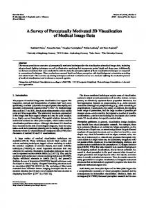
Shape matching through nonrigid shape deformation is a typical approach to measure shape similarity [6, 14, 10, 21, 13, 16]. In general, this approach measures the amount of energy required to deform one shape contour into another based on some physical or mathematical model. The model is then optimized using methods such as dynamic programming to obtain a set of corresponded points on the two shape contours that minimize the deformation cost of this model. However, this approach is often very sensitive to strong, local shape variations that human vision may handle very well. For example, the two shape contours shown in Figs. 1(a) and (b) are similar in general, but their outward parts, represented by the dashed curves, are quite different from each other. A large deformation cost may be required to match these two shape contours.

1. Introduction (a)

Accurately and reliably measuring the similarity of two shape instances is a fundamental problem in computer vision and plays a central role in many shape-based vision applications including shape matching, shape classification, shape recognition, and shape retrieval. From 2D images, closed contours aligned with object boundaries can be extracted as shape instances, which we also refer to as shape contours. These extracted shape contours may demonstrate a large amount of variation, have highly articulated shape parts, involve global and/or local non-rigid deformations, and contain partial occlusions. Even with such complexities, human vision can easily determine whether two shape contours belong to the same shape class. However, developing computational models and methods that can accomplish the same task has proven to be challenging.

(b)

(c)

(d)

Figure 1. (a-b) Shape contours with strong local variations that may show low similarity using a deformable shape matching method. (c-d) Shape contours with small structural changes that may show low similarity using a medial axis matching method.

Another approach is to decompose each shape contour into a set of shape parts [9, 24, 22]. This is typically achieved by determining the medial axes of the shape contour and then constructing a medial-axis tree, where a subtree may represent a shape part. Using this approach, two shape contours are similar when their medial axis trees are structurally similar. In this case, the shape instances illustrated in Fig. 1 (a-b), may be well-matched because the medial axes of the two shape instances are very similar. However, medial axis identification is very sensitive to the

noise along the shape contour. For example, the shape contour shown in Fig. 1(d) is a slightly varied version of the shape contour shown in Fig. 1(c), but their medial axes, represented by the dashed curves, have completely different structures. In this paper, we introduce two new, perceptually motivated strategies for improving the performance of shape classification.

1.1. Overview of Strategy I The first strategy aims to better handle the shape contours that contain thin, elongated strand structures. Such strand structures may point inward or outward. Two examples of shape contours with outward strand structures are shown in Fig. 2(a) and (b), and an example of a shape contour with inward strand structures is shown in Fig. 2(e).

(a)

(b)

(c)

(d)

ing inward strand structures, we obtain a base structure as illustrated in Fig. 2(f), which is actually the union of the extracted inward structures and the original shape contour. When the inward strand structures are small compared to the structure described by the original shape contour, its removal does not affect the general human perception of the shape contour. For example, humans usually perceive the shape contours in Fig. 2(e) and (f) to be of the same shape class. This observation motivates us to handle such shape contours by extracting and removing the inward structures before shape matching and classification. Besides the perceptual motivation, this strategy actually combines the merits of both the deformable shape-matching methods and the medial-axis-based structure matching methods mentioned above. The reasons are twofold: (a) instead of a general shape decomposition for consistent shape components (which is very sensitive to local shape variation) we only use shape decomposition to identify thin, elongated strand structures, which can be done robustly and accurately, and (b) the base structures are simpler and have fewer local variations than the original shape contour. Therefore, the similarity of base structures can be more accurately and robustly estimated by using a deformable shape-matching method.

1.2. Overview of Strategy II (e)

(f)

Figure 2. (a-b) Two shape contours with outward strand structures. (c-d) Base structure and strand structures of (a) after shape decomposition. (e) A shape contour with inward strand structures. (f) Base structure of (e) after removing inward strand structures.

In practice, outward strand structures usually describe “leg” or “branch”-like shape components. In human perception, the exact geometry, such as the curvature and length of strand structures, may not be important for shape recognition and classification. For example, the shape contours shown in Fig. 2(a) and (b) are of the same shape class (octopus) and demonstrate high shape similarity in human perception although their legs may be quite different from each other in terms of geometry and size. This observation motivates us to handle such shape contours by decomposing them into a base structure and a set of strand structures, as illustrated in Fig. 2(c) and (d) respectively. When evaluating the similarity between two such shape contours, we can match their base structures and strand structures separately. In particular, we apply a deformable shape matching method to compare base structures. When matching strand structures, we simply check whether these two shape contours have a similar number of strands, omitting their detailed geometry. Inward strand structure can also be extracted by shape decomposition (to be detailed in Section 2). By remov-

The second strategy aims to better handle shape contours that show good bilateral symmetry. For such a shape contour, a certain level of scaling along its symmetric axis or the direction perpendicular to its symmetry axis usually does not change the human perception of its shape. For example, the three different shape contours shown in Fig. 3(a) (b) and (c) all belong to the same shape class (tree) in human perception. This motivates us to handle such shape contours by identifying their symmetry axes and unifying their aspect ratio before quantitatively evaluating their shape similarity. Here we define the aspect ratio of a symmetric shape contour to be the ratio between the length and width of its bounding box along the symmetry axis, as illustrated in Fig. 3(a). Strategies I and II can be used together to further improve performance.

2. Proposed Method In this section, we describe algorithms to implement the two strategies discussed in Sections 1.1 and 1.2.

2.1. Algorithm for Strategy I In this paper, we consider a shape component to be a strand structure only if it satisfies three criteria: (a) it is a branch attached to a single base structure, (b) it is of relatively small size compared with the original shape struc-

length

symmetry axis

width

(b) (c) (a) Figure 3. (a) A shape contour with good bilateral symmetry. Its symmetry axis is shown with a dashed line and its bounding box is shown with a dotted line. (b) The shape contour produced by scaling (a) along the direction that is perpendicular to its symmetry axis. (c) The shape contour produced by scaling (a) along its symmetry axis.

ture, and (c) it is thin and elongated. For example, the dashed curves in Fig. 4(a) describe two outward strand structures and the dashed curve in Fig. 4(b) describes an inward strand structure. However, the thin, elongated part shown in Fig. 4(c) is not considered to be a strand structure because it is not a branch of the shape and is not attached to a single base structure. The three thin, elongated parts shown in Fig. 4(d) are also not considered to be strand structures because they constitute a considerable area of the original shape structure. If we treat them as three strand structures, the remaining base structure would be too small to contain meaningful information for shape matching.

criteria (b) and (c) as strand structures. The remaining structure after removing all the strand structures is the base structure. Criterion (b) is satisfied if the ratio between the area of the considered candidate strand structure and the area inside the original shape contour is larger than a preset threshold tR . Criterion (c) is satisfied if the ratio between the length and width of the considered candidate strand structure, as illustrated Fig. 4(e), is larger than a preset threshold tL . To identify outward strand structures, we carry out shape decomposition on the original shape contour. This is done by first triangulating the shape contour and connecting the centers of each triangle to construct a medial-axis tree [12]. Specifically, given a shape contour S, we sequentially and uniformly sample n points P = {pi , i = 1, . . . , n}, where pi = (xi , yi ) represents the ith point along S. The points in P are then triangulated into a set of triangles T = {Tk , k = 1, . . . , n − 2}, as illustrated in Fig. 5(a). By defining the center of each triangle in T as a node, we can construct a dual graph GT = (VT , ET ) [7], as shown by the red curves in Fig. 5(b), which is a tree describing the medial axis of the original shape contour.

16 5

(a) 18

17

width

(b) 18

17 19

19

16

16 5 4

5

7

6

4

7

6

20 1

area

14

15

2 10

8

1

14

2 8

9

10

9

length 12

12 13

(a)

20

3

3 15

(b)

(c)

11

13

11

(d)

Figure 5. (a) Triangulation of a fly shape contour, (b) a dual graph, i.e., medial axis (red curves), constructed from (a), (c) feature (red) and leaf (blue) triangles, and (d) a shape tree constructed from the feature and leaf triangles.

(c)

(d)

(e)

Figure 4. (a-b) Example shape contours with strand structures, (cd) example shape contours without strand structures, and (e) the area, length, and width of a candidate strand structure, used for determining a strand structure.

In this algorithm, we use a shape-decomposition algorithm to first identify all the shape branches as candidate strand structures and then select only candidates that satisfy

Given that each node in VT represents a triangle in T , further inspection reveals that each triangle in T can be grouped into one of three categories: triangles with one neighboring triangle, triangles with two neighboring triangles, and triangles with three neighboring triangles. For the purposes of this paper, we will denote triangles with three neighbors as feature triangles and triangles with one neighbor as leaf triangles, which are illustrated as red and blue triangles in Fig. 5(c) respectively. We then construct a shape tree G = (V, E) using only the nodes in VT that represent

feature and leaf triangles, as shown in Fig. 5(d), where each edge e = (u, v) ∈ E indicates that there is a unique path between two nodes u and v in GT . We also denote the nodes in V that represent feature triangles as feature nodes, and the nodes in V that represent leaf triangles as leaf nodes. We define the length of this edge to be the length of the corresponding path in GT . For example, the edge length between nodes 5 and 16 in Fig. 5(d) is length of the red path between points 5 and 16 (shown as red dots) in Fig. 5(b). In the shape tree, each path that links a leaf node uL and a feature node uF represents a candidate strand structure. We simply check each of these candidates using the above criteria (b) and (c) to determine the final strand structures. The length of a candidate strand structure is the length of the corresponding edge in G and the width of a candidate strand structure can be estimated by averaging the circumradii of the triangles in T along the path between uL and uF . To identify inward strand structures, we triangulate the complement of shape contour S. More specifically, we construct a square (or circular) boundary around S, as shown in Fig. 6(b) and triangulate the region between S and this surrounding boundary. However, this region will not be simple, which leads to a shape tree with cycles. To address this problem, we find the closest pair of points between S and the surrounding boundary, connect them into a line segment, and then remove a strip around the line segment from the region between S and the surrounding curve. The resulting region is simple and can be triangulated, as shown in Fig. 6(b), to construct the acyclic medial axis and shape tree, as shown in Fig. 6(c). The remaining work of identifying inward strand structures is exactly the same as the above-mentioned algorithm for identifying outward strand structures. 10

9 5

4 6

11 12

1

2

(a)

(b)

3 8

7

(c)

Figure 6. (a) A shape contour S with an inward strand structure. (b) Construct the complement of S by introducing a surrounding boundary. A strip region at the middle left side is removed before triangulation. (c) The constructed shape tree for identifying inward strand structures.

is invariant under rotation, translation, and (uniform) scaling transformations to any one of these two shape contours. Also assume that the shape decomposition algorithm for identifying outward strand structure decomposes Si into a base structure Ei and ni outward strands, and the shape decomposition algorithm for identifying inward strand structure decomposes Si into a base structure Fi (i = 1, 2) and some inward strands. We use the following voting algorithm to update the match cost C(S1 , S2 ) to φ1 (S1 , S2 ) =

min{C(S1 , S2 ), C(E1 , E2 ) · c(n1 , n2 ), C(F1 , F2 )},

where c(n1 , n2 ) = 1 if the outward strand structures identified from S1 and S2 match well and c(n1 , n2 ) = ∞ otherwise. In all our experiments, we simply make c(n1 , n2 ) = 1 when both ni ≥ 2, i = 1, 2, which indicates that both shape contours contain noticeable number of outward strand structures.

2.2. Algorithm for Strategy II The second strategy handles shape contours that show bilateral symmetry [8, 30, 3]. In this paper, we employ a simple exhaustive search algorithm to check whether a shape contour S is symmetric and if so, identify its symmetry axis. As in Strategy I, a set of n points P = {pi , i = 1, . . . , n} are first uniformly sampled along S. For each pi , we find the corresponding midpoint q ¯i when traversing S starting from and ending at pi . In a small neighborhood around q ¯i , we sample a set of points qi1 , qi2 , . . . , qim on S surrounding q ¯i , as illustrated in Fig. 7(a). Each line pi qik splits l r S into two parts Sik and Sik , k = 1, 2, . . . , m representing the left and right halves respectively. We then mirror l l against the line pi qik to get S˜ik . We denote the region Sik l l and the region bounded by S˜ik and the line pi qik to be Rik r r bounded by Sik and the line pi qik to be Rik . We measure the likeliness of pi qik being a symmetry axis of S by the Jaccard coefficient, ρ(pi qik ) =

l r |Rik ∩ Rik | , l r |Rik ∪ Rik |

(1)

where | · | calculates the region area. Among all n × m candidate symmetry axes pi qik , i = 1, 2, . . . , n; k = 1, 2, . . . , m, we find the one with the maximal axis likeliness (1), ρ(ps qst ) ≥ ρ(pi qik ),

This strand identification algorithm can be incorporated into any available shape classification method to improve performance. Assume that we have arbitrarily choosen such a method which can provide us with a matching cost C(S1 , S2 ) for any two shape contours S1 and S2 . This matching cost negatively measures the shape similarity and

∀i = 1, 2, . . . , n; k = 1, 2, . . . , m. If ρ(ps qst ) is larger than a given threshold tρ1 ∈ [0, 1], we consider S to be a symmetric shape, with a symmetry axis ps qst . We then find the line Nst that is normal to ps qst and passes the midpoints of the line segment ps qst . We

qi1

qi

pi

qim

(a)

(b)

Figure 7. An illustration of shape symmetry detection in Strategy II. (a) Exhaustively searching for the symmetry axis of a shape contour. (b) An example of a shape with two perpendicular symmetry axes.

further check the axis likeliness of Nst : if ρ(Nst ) is larger than a given threshold tρ2 ∈ [0, 1], we claim that Nst is another symmetry axis of S. In this strategy, we only handle shape contours S with a single symmetry axis, i.e., S satisfies ρ(ps qst ) > tρ1 and ρ(Nst ) ≤ tρ2 . For shape contours that are also symmetric against Nst , as illustrated in Fig. 7(b), we do not apply Strategy II because the aspect ratio of the the shape contour may not be uniquely defined. Given two shape contours S1 and S2 , if we can identify a single symmetric axis, say l1 and l2 , from each contour, we unify their aspect ratio before evaluating their shape similarity. In particular, we treat one of them, say S1 , as the template and the other one, S2 , as the target. We can find a unique bounding box (i.e., a rectangle) for each by requiring that one side of the bounding box be parallel to the identified symmetry axis, as illustrated in Fig. 8(a) and (b). We then scale the target shape contour S2 along its symmetry axis to a shape contour S2 such that it has the same aspect ratio as the template, as illustrated in Fig. 8(c). Given an available shape-classification method that measures the matching cost C(S1 , S2 ) between S1 and S2 , we update the matching cost to φ2 (S1 , S2 ) = min{C(S1 , S2 ), C(S1 , S2 )}. Note that if either S1 or S2 are not symmetric or contain a second symmetry axis that is normal to the first symmetry axis, we simply set φ2 (S1 , S2 ) = C(S1 , S2 ) without applying Strategy II. To use Strategy I and Strategy II together, we simply combine the matching costs to obtain φ(S1 , S2 ) = min{φ1 (S1 , S2 ), φ2 (S1 , S2 )}.

3. Experiments We implement the previously-discussed methods in C++ using the OpenCV library. Contour triangulation from a set of sampled points is implemented using the software developed by Shewchuk [23]. We selected the Inner Distance

(a)

(b)

(c)

Figure 8. (a-b) Two different symmetric shape contours and their bounding boxes. (c) Scaling the shape contour (b) along its symmetric axis to make its aspect ratio identical to the aspect ratio of shape contour (a).

Shape Context (IDSC) method [16] to measure the shapematching cost C(S1 , S2 ) between two shape contours S1 and S2 , largely because the source code is readily available online. Recently, Yang et al. [31] developed a new approach to classify a large set of shape contours by extending pairwise shape matching to group-wise shape matching in an unsupervised fashion. For this approach, a locally constrained diffusion process (LCDP) was developed to enhance the similarity of two shape contours if they have low matching cost with another shape contour. The LCDP method also uses the IDSC method for measuring the pairwise shape similarity. LCDP achieves state-of-the-art shape classification performance on several well-known data sets. In our experiments, we attempt to show that the proposed strategies can improve the performance of IDSC and, by using IDSC augmented with the proposed strategies as the pairwise matching method, the performance of LCDP can be further improved. In all our experiments, we uniformly sample n = 256 points on each contour. For Strategy I, we set the area threshold tR = 0.12, and the length-width threshold tL = 3.0 for identifying outward structures and tL = 6.0 for identifying inward structures. For Strategy II, we set the axis likeliness thresholds tρ1 = 0.74 and tρ2 = 0.68.

3.1. MPEG-7 Data Set We first test the proposed method on the widely used MPEG-7 data set (specifically the MPEG-7 CE-Shape-1 Part B) [15] that defines 70 shape classes, where each shape class contains 20 different shape contours in the form of binary images. In total, the MPEG-7 data set contains 1, 400 shape contours. A subset of the shape classes are illustrated in Fig. 9. We use Bullseye testing to evaluate the performance of the shape classification. In this test, a shape contour is selected from the data set as the template, and matched to all 1, 400 shape contours in this data set. The 40 most similar shape contours (i.e. with the smallest matching cost) are selected, and out of these 40, we count the number of shape contours that are actually in the same shape class

as the template. This number is divided by 20 (the number of shape contours in the template class) to obtain a classification rate. This process is repeated by taking each of the 1, 400 shape contours as the template and obtain an average classification rate as the performance.

Figure 9. Subset of shape classes in the MPEG-7 data set.

Table 1 shows the Bullseye testing results on the MPEG7 data set using the original IDSC method [16], the original LCDP method [31] 1 , the IDSC and LCDP methods augmented with the proposed strategies, and other recently published methods. By using the proposed strategies, the shape classification rate of IDSC is improved from 85.40% to 88.39% and the shape classification rate of LCDP is improved from 92.36% to 95.60%. Table 2 compares the classification rate when using only Strategy I, only Strategy II and both Strategy I and II together. Figure 10 shows several examples of the shape contours in the MPEG-7 data set that are decomposed into base and strand structures by using Strategy I. Figure 11 shows several examples of the symmetric shape contours in the MPEG-7 data set as determined by Strategy II.

Method Proposed method + IDSC + LCDP IDSC + LCDP + unsupervised GP [31] IDSC + LCDP [31] IDSC + LP [5] Contour Flexibility [29] Proposed method + IDSC Shape-tree [13] Triangle Area [2] IDSC(EMD) [17] Hierarchical Procrustes [18] Symbolic Representation [11] IDSC [16] ˆ Rouge [20] Shape L’Ane Multiscale Representation [1] Polygonal Multiresolution [4] Fixed Correspondence [27] Chance Probability Function [26] Curvature Scale Space [19] Generative Model [28]

Rate 95.60 % 93.32 % 92.36 % 91.61 % 89.31 % 88.39 % 87.70 % 87.23 % 86.56 % 86.35 % 85.92 % 85.40 % 85.25 % 84.93 % 84.33 % 84.05 % 82.69 % 81.12 % 80.03 %

Table 1. Shape classification rate on the MPEG-7 data set.

Method IDSC [16] Strategy I + IDSC Strategy II + IDSC Strategy I&II + IDSC IDSC + LCDP [31] Strategy I + IDSC + LCDP Strategy II + IDSC + LCDP Strategy I&II + IDSC + LCDP

Rate 85.40 % 87.68 % 86.41 % 88.39 % 92.36 % 94.85 % 93.80 % 95.60 %

Table 2. Shape classification rate on the MPEG-7 data set, when using only Strategy I, only Strategy II, and both Strategy I and II.

Figure 10. Example strand structures, and base structures found by the proposed method. The red curves represent the inward or outward strand structure, and the black curve represents the base structure.

3.2. Brown Database Additionaly, we apply the proposed method to the Brown database [22], specifically the second database, that defines 1 Yang et al also report results of 97.21% on the MPEG-7 data set using supervised ghost points. In this paper our focus is on unsupervised methods.

Figure 11. Example symmetric shape contours in the MPEG7 data set. Symmetric axes are shown in green.

Method Proposed method + IDSC + LCDP IDSC + LP [5] Shape-tree [13] IDSC [16] Shock-Graph Edit [22] Generative Models [28]

1st 99 99 99 99 99 99

2nd 99 99 99 99 99 97

3rd 99 99 99 99 99 99

4th 99 99 99 98 98 98

5th 99 99 99 98 98 96

6th 99 99 99 97 97 96

7th 99 99 99 97 96 94

8th 99 99 97 98 95 83

9th 99 97 93 94 93 75

10th 99 99 86 79 82 48

Table 3. Shape classification result on the Brown database.

Method IDSC [16] Strategy I + IDSC Strategy II + IDSC Strategy I&II + IDSC

1st 99 99 99 99

2nd 99 99 99 99

3rd 99 99 99 99

4th 98 98 98 98

5th 98 99 98 99

6th 97 99 97 99

7th 97 99 97 99

8th 98 97 98 97

9th 94 96 94 96

10th 79 84 79 84

Table 4. Shape classification results on the Brown data set, when using only Strategy I, only Strategy II, and both Strategy I and II.

9 shape classes as illustrated in Fig. 12, where each shape class contains 11 different shape contours in the form of binary images. In total, the Brown database contains 99 shape contours. As in [13, 5, 16], Table 3 reports the performance as follows: one shape contour is selected from the data set as the template and then matched to the remaining shape contours. The top 10 best matches are checked and only matches that are in the same shape class as the template are counted as correct matches. This process is repeated by taking each one of the 99 shape contours in the whole data set as the template. Then we check the total correct matches for the i-th contour, i = 1, 2, . . . , 10, which are shown in Table 3. Note that the maximum possible correct matches in total for the i-th contour is 99. We can see that the LCDP method, when augmented with the proposed two strategies, achieves the maximum correct matches for each contour selected as the template. Table 4 shows the results on this data set by applying Strategy I, Strategy II and both Strategy I and II to IDSC.

Figure 12. The nine shape classes in the Brown database.

from which we can see that the integration of the proposed strategies does not introduce significant improvement over LCDP [31]. The reasons are twofold. First, the leaf shape contours in this data set do not contain multiple strand structures. Second, most leaves in the same species are of a similar aspect ratio. Therefore, the proposed strategies do not introduce significant overall change to the original matching cost of LCDP (or IDSC) and cannot further improve the shape classification performance.

Figure 13. The fifteen leaf species in the Swedish leaf data set.

Method Proposed Method + IDSC+ LCDP IDSC + LCDP [31] Shape-tree [13] IDSC [16]

Rate 98.27 % 98.20 % 96.28 % 94.13 %

3.3. Swedish Leaf Data Set The Swedish leaf data set [25] contains isolated leaves from 15 different Swedish tree species, with 75 leaves per species. Examples from the 15 leaf species are shown in Fig. 13. As in [16, 13, 31], we use the 1-nearest-neighbor approach to measure the classification performance for this data set where, for each leaf species, 25 samples are selected as a template and the other 50 are selected as targets. Shape classification results on this data set are shown in Table 5,

Table 5. Shape classification rate on the Swedish leaf data set.

4. Conclusion In this paper, we have suggested two new, perceptually motivated strategies to improve shape similarity measures and shape classification performance. In Strategy I, we decompose a shape contour into a base structure and a set

of inward or outward strand structures. We have shown that the similarity of two such shape contours can be better modeled by measuring the similarity of their base structures and the similarity of their respective strand structures in different ways. In Strategy II, we unify the aspect ratio of the the symmetric shape contours before evaluating their shape similarity. Experiments on the widely used MPEG-7, Brown, and Swedish leaf data sets illustrate that the proposed strategies can improve the state-of-the-art shape classification performance.

Acknowledgement The authors would like to thank Haibin Ling for providing the code for IDSC and Xingwei Yang for providing the code for LCDP. This work was funded, in part, by AFOSR FA9550-07-1-0250 and NSF IIS-0951754.

References [1] T. Adamek and N. E. O’Connor. A multiscale representation method for nonrigid shapes with a single closed contour. IEEE Trans. Circuits and Systems for Video Technology, 14(5):742–753, 2004. [2] N. Alajlan, M. S. Kamel, and G. H. Freeman. Geometrybased image retrieval in binary image databases. IEEE TPAMI, 30(6):1003–1013, 2008. [3] M. Atallah. On symmetry detection. IEEE Trans. on Computers, 34:663–666, 1985. [4] E. Attalla and P. Siy. Robust shape similarity retrieval based on contour segmentation polygonal multiresolution and elastic matching. Pattern Recognition, 38(12):2229–2241, December 2005. [5] X. Bai, X. Yang, L. J. Latecki, W. Liu, and Z. Tu. Learning context sensitive shape similarity by graph transduction. IEEE TPAMI, 2009. [6] R. Basri, L. Costa, D. Geiger, and D. Jacobs. Determining the similarity of deformable shapes. Vision Research, 38:135–143, 1998. [7] M. Berg, O. Cheong, M. van Kreveld, and M. Overmars. Computational Geometry Algorithms and Applications. Springer, 2008. [8] K. Bitsakos, H. Yi, L. Yi, and C. Fermuller. Bilateral symmetry of object silhouettes under perspective projection. In ICPR, 2008. [9] H. Blum. Biological shape and visual science. Theoretical Biology, 38:205–287, 1973. [10] J. Coughlan, A. Yuille, C. English, and D. Snow. Efficient deformable template detection and localization without user initialization. CVIU, 78(3):303–319, 2000. [11] M. R. Daliri and V. Torre. Robust symbolic representation for shape recognition and retrieval. Pattern Recognition, 41(5), 2008. [12] P. F. Felzenszwalb. Representation and detection of deformable shapes. IEEE TPAMI, 27(2):208–220, 2005. [13] P. F. Felzenszwalb and J. D. Schwartz. Hierarchical matching of deformable shapes. In IEEE CVPR, 2007.

[14] U. Grenander, Y. Chow, and D. Keenan. Hands: a pattern theoretic study of biological shapes. Springer-Verlag New York, Inc., New York, NY, USA, 1991. [15] L. Latecki and R. Lakaemper. Shape similarity measure based on correspondence of visual parts. IEEE TPAMI, 22(10):1–6, October 2000. [16] H. Ling and D. W. Jacobs. Shape classification using the inner-distance. IEEE TPAMI, 29(2):286–299, 2007. [17] H. Ling and K. Okada. An efficient earth mover’s distance algorithm for robust histogram comparison. IEEE TPAMI, 29(5):840–853, 2007. [18] G. Mcneill and S. Vijayakumar. Hierarchical procrustes matching for shape retrieval. In IEEE CVPR, pages 885– 894, 2006. [19] F. Mokhtarian and M. Bober. Curvature Scale Space Representation: Theory, Applications, and MPEG-7 Standardization. Kluwer Academic Publishers, Norwell, MA, USA, 2003. [20] A. M. Peter, A. Rangarajan, and J. Ho. Shape l’ane rouge: Sliding wavelets for indexing and retrieval. In IEEE CVPR, 2008. [21] T. B. Sebastian, P. N. Klein, and B. B. Kimia. On aligning curves. IEEE TPAMI, 25(1):116–125, 2003. [22] T. B. Sebastian, P. N. Klein, and B. B. Kimia. Recognition of shapes by editing their shock graphs. IEEE TPAMI, 26(5):550–571, 2004. [23] J. R. Shewchuk. Triangle: Engineering a 2D Quality Mesh Generator and Delaunay Triangulator. In Applied Computational Geometry: Towards Geometric Engineering, volume 1148 of Lecture Notes in Computer Science, pages 203–222. Springer-Verlag, 1996. [24] K. Siddiqi, A. Shokoufandeh, S. J. Dickinson, and S. W. Z. Y. Shock graphs and shape matching. IJCV, 35:13–32, 1999. [25] O. J. O. S¨oderkvist. Computer vision classification of leaves from swedish trees. Master’s thesis, Link¨oping University, SE-581 83 Link¨oping, Sweden, September 2001. LiTH-ISYEX-3132. [26] B. Super. Learning chance probability functions for shape retrieval or classification. In CVRP Workshop on Learning in Computer Vision and Pattern Recognition, 2004. [27] B. Super. Retrieval from shape databases using chance probability functions and fixed correspondence. International Journal of Pattern Recognition and Artificial Intelligence, 20(8):1117–1138, 2006. [28] Z. Tu and A. L. Yuille. Shape matching and recognition using generative models and informative features. In ECCV, pages 195–209, 2004. [29] C. Xu, J. Liu, and X. Tang. 2d shape matching by contour flexibility. IEEE TPAMI, 31(1):180–186, 2009. [30] X. Yang, N. Adluru, L. Latecki, X. Bai, and Z. Pizlo. Symmetry of shapes via self-similarity. In International Symposium on Visual Computing, pages II: 561–570, 2008. [31] X. Yang, S. Koknar Tezel, and L. Latecki. Locally constrained diffusion process on locally densified distance spaces with applications to shape retrieval. In IEEE CVPR, pages 357–364, 2009.