Two-channel Separation of Speech Using Direction-of-arrival Estimation And Sinusoids Plus Transients Modeling Mikko Parviainen1 and Tuomas Virtanen2 Institute of Signal Processing Tampere University of Technology, P.O. BOX 33101, Tampere, Finland 1 E-mail:
[email protected] 2 E-mail:
[email protected] Abstract: In this paper a sound source separation system operating in real-world acoustic environments is proposed. Two signals are recorded using sensors which are placed close to each other. The separation is based on the spatial origin of sound sources. The overall system consists of two separate parts. In the first part the direction-of-arrival of the strongest sound source is estimated. The second part performs the separation of the sound source by sinusoids + transients representation which allows grouping of spectral components based on estimated direction-of-arrival. The operation of both parts is based on the time delay between the channels, which is related to the spatial origin of sound sources. Grouping of transients is proposed as a novel separation method. The simulations performed with the system showed that the separation is possible using the selected approach.
1. Introduction Sound source separation in general refers to signal processing techniques, the goal of which is to isolate one or several sound sources from a mixture signal which contains desired sound sources and undesired sound sources. The sound source separation has received a lot of attention over the years. Solely in audio signal processing, several drastically differing models have been proposed. But there are also numerous applications directed to everyday life of people and to other scientific purposes in which a system capable of separating the desired sound source is useful. Human auditory system is able to separate sound sources tremendously well. This ability is often referred to as cocktail-party effect. The term was introduced by Cherry as early as in 1950s from the basis of his experiments in which the concentration on single talker speech in the presence of several other talkers was studied. In many cases mixture signals consist not only of clean source signals but also background noise. From this viewpoint it is easy to understand that picking only one of the signals in the mixture introduces a very challenging task. Despite the fact that area of sound source separation has been studied for decades, still, the currently employed schemes are merely rather theoretically oriented. Human auditory system has the ability to separate sound sources in rather challenging auditory conditions. Bregman [2] lists the following association cues in human auditory organization: (1) spectral proximity, (2) harmonic concordance, (3) synchronous changes of the components (common onset/offset, common amplitude/frequency modulation), (4) spatial proximity. In this system, spatial proximity is used as the only cue of grouping spectral components. Therefore, the sources are assumed to locate spatially apart from each other. Several solutions for sound source separation have been proposed over the years. Many of them try to
separate sound sources from one-channel data. In general these separation systems do not work in the case of real-world signals. Human auditory system is able to separate sound sources using two-channel data thus, it is interesting to find out that can a separation machine be built that is able to perform at least to some extent similar to human hearing. There are also multi-channel solutions which utilize for instance 10-channel data. 1. 1 System overview The main hypothesis in this system is that the spatial information related to sound sources is the main cue based on which the separation can performed in real-world environments. The hypothesis, as well as, the solutions for sound source separation arise from the previous research done in the area, meaning, no fundamentally new ideas are proposed but the existing knowledge and approaches are utilized and ideas from different research areas are merged. The proposed separation algorithm requires a receiver unit which is fixed in advance. Sound sources are assumed to be spatially apart, that is, only one sound source exists at certain horizontal angle. The signals are recorded using two equal microphones which are at the same height, placed at small distance from each other. The sound source separation consists of the following main steps: (1) The locations of sound sources are determined, (2) input mixture is modeled using sinusoids + transients representation, (3) the components of the modeled mixture are grouped based on the location information, and finally, (4) the components from the desired sound source are synthesized. This process in illustrated in Figure 1. Nakatani and Okuno have proposed a system in which direction-of-arrival (DOA) was used as a supplementary grouping cue in the grouping of sinusoidal components [6]. In our system the grouping is fully based on DOA information. In addition to sinusoids, also detected transients are grouped. Due to the fact that the system is utilized in realworld environments, the location of sound sources should be determined in three planes: horizontal plane, median plane and frontal plane. For a fixed location of the receiver, the estimation of the horizontal angle ϕ and elevation angle uniquely define DOA in three dimensional space. Yet, to determine the unique location of a sound source the distance has to be estimated. In the separation system sound sources are assumed to be located in horizontal plane, that is, only ϕ needs to be estimated. This is the initial evaluation of sound source separation based on the architecture in Figure 1. The estimation of horizontal angle is based on the time delay between the left and right channel signals. The estimation algorithm is explained in Section 2. The elevation angle and the distance of a sound source are not needed in the separation and they are thus not estimated. Left and right channel signals are modeled using the
Analysis stage
DOA estimator
Grouping stage
Synthesis stage
source location parameters of admissible sinusoids parameters of sinusoids
mixture signal (left and right channel)
delay
sinusoids + transients modeling
parametric sinusoid generator separated signal
thresholding unit transient locations
+ transient locations transient port
delay
Figure 1. System block diagram
sinusoids + transients mid-level representation which is described in Section 3. The representation enables signal separation by the DOA estimate, that is, time delay between left and right channel. Using the estimated time delay, the elements of the mid-level representation are grouped to sources which can be synthesized separately. The details concerning these stages can be found in Section 4. and in Section 5. Despite the fact that sound source separation is the ultimate goal, using directionof-arrival as a primary cue, the DOA subsystem has to be selected carefully.
2. Direction-of-arrival Estimation The preliminary requirements for the DOA system with a particular measurement setup are the following: (1) operate reliably on data recorded in real-world environments, (2) handle arbitrary signal contents, (3) make no assumptions concerning environment. It is worth pointing out that DOA systems in general do not perform either reliably or accurately with two-sensor setups. Instead, advanced signal processing techniques have to be utilized. A DOA system that largely fulfills the requirements is introduced by Liu et al. in [3]. Our system contains certain simplifications and modifications to make it more usable for the purposes of this work. However, the basic structure is exactly the same. The system utilizes the same principles as the early models of human hearing (discussion on the models can be found in [1] and in [7]). The system obeys coincidence detection principle in localization of sound sources. The estimation of the sound source location is based on delaying the left channel signal respect to the right channel or vice versa. The time delay which results in the best match between the signals corresponds to a certain spatial location and can be mapped to a horizontal angle ϕ. The delay is estimated in each frame to each frequency component. The robustness of the estimate is improved by integrating it over time and frequency. The formula in the following discussion apply to one frame. The best match between two input signals is found by feeding a coincidence detection system by Sl (m) and Sr (m) which are short-time Fourier transforms (STFT) of respective discrete time signals sl (k) and sr (k). STFTs of delayed time domain signals can be expressed by multiplying original STFTs by a complex exponential: m Sli (m) = Sl (m)exp(−j2π fs τi ) M m Sri (m) = Sr (m)exp(−j2π fs τI −i+1 ) (1) M m = 0, . . . , M /2 − 1 i = 1, . . . , I where Sli (m) is the STFT of the left channel delayed
with the time delay τi and Sri (m) is the STFT of the right channel delayed with the time delay τI −i+1 . I variants of STFTs are produced by Equation (1) for each channel. Next, each variant is compared between left and right channel. For each time delay τi : i = 1, . . . , I, a distance measure is formed. This is described by Equation (2). ¯ ¯ ¯ ¯ ∆S i (m) = ¯Sli (m) − Sri (m)¯ (2) m = 0, . . . , M /2 − 1 i = 1, . . . , I where ∆S i (m) is the distance measure which enables the actual comparison. The output of this stage is obtained by picking the minimum of the sequence ∆S i (m) : i = 1, . . . , I and recording its place in the delay line, that is, the index i. The remaining stages of the DOA estimation system improve the reliability of the detection mechanism by integrating the estimated delays over time and frequency. The robustness against spurious responses occurring especially in natural environments and multi-source cases is achieved. Finally, the delays i are mapped to horizontal angle ϕ. The relation between the horizontal angle ϕi and the discrete delay i is defined by Equation (3). π i−1 ϕi = − π 2 I −1
(3)
The details concerning the DOA estimation system can be found in [7].
3. Sinusoids + Transients Modeling Left and right channel are modeled using the sinusoids plus transients representation. The representation allows grouping of spectral components based on the estimated DOA, as described in Section 4. Sinusoidal modeling was presented by McAulay and Quatieri in [5] for speech coding purposes. Smith and Serra introduced practically the same kind of a model for music signals. Their system was published soon after the previously mentioned and it is presented in [10]. Any signal produced by musical instruments or by a physical system may be viewed to consist of two parts; the deterministic part and the stochastic part [9]. The deterministic part can be modeled as a sum of sinusoids. The local signal model is defined by Equation (4). s(t) =
Q −1 X q =0
a(q ) cos[ω (q ) t + θ(q ) ] + r(t)
(4)
where a(q ) is amplitude, ω (q ) frequency and phase θ(q ) of qth sinusoid. r(t) embraces the stochastic part at time instant t. In this particular system sinusoids are assumed to be locally stable, that is, no changes are allowed to occur within a time interval fixed by analysis window. This is of course not true in a general case but on the other hand it is not totally unreasonable assumption since the time interval is usually small. In fact, deterministic + stochastic models in general assume that sinusoids do not exhibit rapid changes. However, slow variations of amplitudes and frequencies are allowed over analysis window [9]. The sinusoidal model is most efficient in the case of periodic sounds. For perceptually important shortduration transients it performs poorly. Therefore, a transient model is applied to model these parts of a signal. The idea of using a separate model for transients in addition to the sinusoidal model was proposed by Levine [4]. His system is meant for audio coding, but the same ideas are utilized in our separation system, too. 3. 1 Sinusoids The sound separation algorithm does not require any specific way to estimate the sinusoids, and basically any algorithm which estimates amplitudes, frequencies and phases in each frame can be used. The most important stages in the analysis of the sinusoids are (1) sinusoid detection and (2) parameter estimation. Various algorithms have been proposed to both stages. In this system a sinusoidal likeness measure [8] (q ) is used to determine frequencies ω{l,r} of sinusoids. The (q ) method is used also to estimate the amplitude a{l,r} and (q ) the phase θ{l,r} of the sinusoid q. The processing is made independently for left channel (l) and right channel (r). 3. 2 Transients There are very few modeling systems that take into account the special role of the transients. This is somewhat surprising since their presence or absence is perceived in listening tests particularly in the case of speech signals. The detection algorithm used in this system is initially proposed by Levine in [4]. The transient detection utilizes the idea of tracking energy changes. In fact, two detection methods are utilized. The first method is a rising edge detector. It searches for rapid changes in signal energy and labels them. The second method requires sinusoidal modeling system with synthesis capability, since it uses also the residual signal. This is not a problem since the output of the sinusoidal analysis is easy to direct to the transient detector. The detection is based on observing the performance of sinusoidal modeling in the current frame. If sinusoidal modeling performs poorly, which is detected by comparing the energy of the residual and the energy of the modeled signal, it is probable that there is a transient in the current frame. The transient detection needs a shorter analysis window than sinusoidal modeling. The duration of a transient is fixed to 64 ms. Constraining the maximum transient rate is done similarly to Levine’s system. The frames corresponding time regions 50 ms before and 150 ms after the frame in which the transient is initially detected, are labeled as non-transient regions. Other
transients detected within this region are considered as invalid. In Levine’s system detected transients, or transient regions, are transform coded. In our system transform coding is not needed but the the output of transient detection system is time instants which define the start and end time of transients.
4. Grouping of Spectral Components In the grouping stage, the sinusoids and transients which belong to the desired sound source are selected. The selection is made by calculating a time difference between left and right channel components, and comparing it to the ideal delay given by the DOA estimate. 4. 1 Sinusoid grouping In the grouping, it is assumed that the desired signal is the same in the left channel and in the right channel. The desired signal in one channel is only delayed compared to the signal received by the other channel. Using the DOA estimate which is obtained for the desired source, the delay can be estimated. On the other hand using the phase information of sinusoids corresponding delay is easily estimated. It is important that a sinusoid picked from the left channel is compared to the correct component in the right channel. In the system this is taken care of by first forming these sinusoid pairs. Those sinusoid pairs for which the delay is near to the delay calculated using the DOA estimate are considered as arising from the desired sound source. The reference information needed to group the sinusoids between the desired part and the undesired part is provided by the DOA estimation system. A DOA estimate has to be converted to a form that enables the phase comparison. The conversion is made by calculating first the time it takes for sound pressure waves to propagate between two sensors, and yet, converting seconds to samples. Time differences are obtained using Equation (5). D sin ϕ (5) c where fs is sampling rate, D is the distance between the sensors, c is propagation speed of sound wave fronts and ϕ is the DOA estimate. Plane wave model is assumed. The grouping of sinusoidal components is based on a phase constraint, which is calculated using the time difference ∆tref . The phase change of a sinusoid in certain time is easily calculated. A frequency component in the left channel is selected, the same component in the right channel is examined by checking how much the phase of the component in the left channel has changed compared to the right channel. The phase difference is (q l) (q r) calculated as ∆θ(q ) = θl − θr , where q {l, r} is the index of a sinusoid in each channel. ∆θ(q ) has to be converted to time difference enabling the grouping. Equation (6) describes the conversion. ∆θ(q ) (6) ∆t(q ) = fs (q ) ω ∆tref = fs
The final decision between the parameter sets that represent the desired part and the undesired part is presented by Equation (7). ½ ¯ ¾ ¯ ¯ ¯ (q ) QD = q| ¯∆t(q ) − ∆tref ¯ < ∆tdev (7) q = 0, . . . , Q − 1
where QD represents the set of elements which consists (q ) of admissible frequency component indices and ∆tdev is a parameter which allows some tolerance to the angle (q ) estimate. ∆tdev is obtained applying Equation (6) and setting the desired tolerance to ϕdev . Several tolerance values were tried and ϕdev = 10◦ was chosen because it was the most suitable to cover all the cases. In general, the more noisy and the more broadband is the signal, the more tolerance is needed. However, one value for the parameter is plausible because it enables the comparison between different environments to some extent. 4. 2 Transient grouping The transients do not have similar parametric representation to sinusoids by which the DOA estimate of a frequency component is easily obtained. However, the instantaneous power of transients is large compared to the interfering sounds so that the spatial origin can be estimated using a broadband DOA system. Let us denote the transient region related to a transient frame by tr{l,r} (g). g = 0, . . . , G − 1 is the index to the detected transients. Note again that both channels are taken into account. First, transient regions tr{l,r} (g) are utilized to find out the absolute locations of transients on time axis from the residual r{l,r} (k) (corresponds r(t) in Equation (4) in discrete-time). Then, for each region tr{l,r} (g) the estimate of DOA ϕtr (g) is obtained by feeding {l,r}
each transient region to the DOA estimation subsystem. Note that the duration of transient regions is sufficient in the sense that DOA system is able to produce plausible estimates. Finally, the grouping between the desired transients and the undesired transients is made based on Equation (8). ¯ ¯ ¾ ¯ ¯ ¯ ¯ tr(g)| ¯ϕtr − ϕ < ϕ ref ¯ dev {l,r} (g)
½ TD =
(8)
where TD represents the set of transients that arise from the estimated horizontal angle ϕref . ϕdev is the maximum allowed deviation from ϕref .
5. Synthesis The sinusoidal synthesis employs overlap-add principle. In general, sinusoidal synthesis is quite straightforward since it is nothing but inserting the estimated parameters; amplitude, frequency and phase to Equation (4), multiplying the synthesized frames by a window function, and summing sequential frames to a contiguous signal. Hamming window function is used and sequential frames overlap by 50% thus the sequential frames sum to unity. However, while considering the final resulting signal the transients have to be taken into account. More precisely, their location information on time axis in each channel has to be available. Using this information, the sinusoidal modeling is turned off and the transient modeling is turned on as the detected transients occur. The transient synthesis consists of simply utilizing the locations of admissible transient regions and copying each transient region to its correct position. Sinusoids and transients in each channel are synthesized thus the resulting signal is also a two-channel signal.
6. Experimental Results The results are presented in two separate parts. The first consists of the estimation of DOA algorithm in various cases. The second part is reserved for a brief discussion of the performance of the separation scheme employed in this system. In order to simulate the performance of the proposed system, test signals were played and recorded in three real-world environments. The measurements took place in an anechoic chamber, a classroom and an office. The anechoic chamber is obviously the easiest case whereas the classroom and the office enabled the evaluation of the algorithms in reverberant environments. In the office environment there were additional noise sources making it the most challenging environment. The setup consisted of two CD-players and two loudspeakers using which the speech signals and the interference signals were played. Two high-quality microphones attached to a stand at the same height were used. The microphones were placed 10 cm apart from each other. In each environment three fundamentally different configurations are evaluated. Case A refers to a configuration in which one sound source is present. The undesired part in a signal mixture received by the sensors thus consists only of the background noise specific to each environment. It should be kept in mind that in addition to the background noise, reflecting surfaces (e.g. walls, floor, ceiling, tables) introduce several weak, but not insignificant, noise sources in rooms in general. Including these interferers, in case B there is a second source acting as a primary interferer. The sound level of the primary interferer is 10 dB weaker measured at receiving end of the configuration compared to the source of interest, and it is placed spatially apart from the desired signal. Case C corresponds best to the classic cocktail-party situation: the source of interest and the primary interferer are equal in loudness. In addition to the recorded signals, a few signal mixtures were generated by delaying the original stimuli in such a way that it corresponds the case in which sound sources are placed at certain horizontal angles. The effect of the room response and the effects introduced by the measurement equipment are not present enabling the evaluation of algorithms in an ideal case. Generated signals also allow better quantitative comparison of the results. 6. 1 Direction-of-arrival Estimation In this work the primary interest is the consistency of DOA estimates. In the case of moving sound source, the estimates before and after the current time instant should experience graceful, or smooth, variation. For instance, a 5◦ or even bigger deviations to the actual horizontal angle are acceptable. Since it is assumed that sources are spatially more distant. Figure 2 presents the DOA estimates in case A and in case C for a two-second excerpts of mixtures. The mixtures are recorded at an office environment. The upper panel presents the performance in case A for a speech signal. It can be stated that the DOA method is able to produce reasonable estimates also for other types of signal. The discussion concerning the signal content as well as the results using various signal contents can be found in [7]. The lower panel in Figure 2 presents DOA estimation performance in a two-talker case (case C). The measurement took place in the same environment as the one-talker case. The fluctuation also in this case is acceptable. In general, DOA estimation based on calculating
25
0
d1: babble d2: speech d3: pop music d4: 1 kHz sinusoid d5: transient sequence d6: white noise
20 15
NSR [dB]
DOA [°]
10
−15
5 0 −5 −10 −15
−30 0
0.5
1 time [s]
1.5
2
60
30 DOA [°]
d1
d2
d3
d4
d5
d6
Figure 3. The energy ratio between a speech signal s(k) and various interfering signals d(k). The first bar is N SRbefore and the second bar is N SRafter .
45
15
0
−15
−30 0
−20
0.5
1 time [s]
1.5
2
Figure 2. Estimated direction-of-arrival for speech signals. The upper panel: The female speaker is at the nominal angle ϕ = −15◦ (case A). The lower panel: The combination male 0 dB at ϕ = −15◦ and female 0 dB at ϕ = 45◦ (case C). Both signals are recorded at an office environment.
cross-correlation between the left channel signal and the right channel signal is possible in the case of one strong sound source. However, in the case of several strong sound sources the method is not able to operate in the desired manner. The DOA estimation method utilized in this work is designed particularly for multi-source cases. 6. 2 Quality of the separated sounds The quantitative performance evaluation is difficult for the recorded signals because the separated speech signal can not be compared to the original speech signal. This is due to the fact that the recorded speech is delayed and attenuated compared to the original speech. Additionally, the recorded signal is affected by room response. Reliable methods to cancel out these factors are not known. However, some performance measures can be calculated using generated mixtures of the original samples that were used in the recordings. Still, these measures give only some kind of a clue of the overall system performance. Generated signals refers to the fact that sound sources are artificially placed at a certain spatial location by delaying the left channel signal compared to the right channel signal or vice versa. The same samples were used to produce the generated mixtures that were used in the measurements. Compared to the recorded signals, the generated mixtures lack the effect of room response which was observed to be significant. The audio quality of the system is affected by a few major factors. If the quality degradation introduced by the signal modeling is ignored, the resulting signal quality is affected by the performance of the grouping stage (see Figure 1). The grouping is performed based on
DOA estimates. Thus, the performance of the DOA subsystem is directly affecting the quality. It was discovered while simulating the subsystems that each performed satisfactorily excluding some special cases. For instance, some tones caused problems to the DOA subsystem. However, broadband stimuli resulted in exact DOA estimates. The effect of the detected transients was studied by comparing the speech signals modeled using only the sinusoidal modeling to the signal which was modeled using not only sinusoids but also the detected transients. In the case of speech signals, virtually all the detected transients are actually consonants in the original signal. The existence of the consonants in the separated signals improves the quality. 6.2. .1 Generated signals The performance of the system is characterized using two values which describe the energy ratio between the interference signal and the speech signal before and after the separation. The observed mixture signal m(k) can be expressed as m(k) = s(k) + d(k), where s(k) is the speech signal and d(k) is the added interference. In this case the ratio is calculated using Equation (9). N SRbefore
P 2 d(k) = 10 log Pk 2 [dB] k s(k)
(9)
The separated signal s˜(k) can be expressed as s˜(k) = s(k) + e(k), where e(k) is the error between the original and separated speech signal, e(k) = s(k) − s˜(k). The energy ratio is now given by Equation (10). P (s(k) − s˜(k))2 N SRafter = 10 log k P [dB] (10) 2 k s(k) If N SRbefore is big, the energy of the source that is considered as an interfering sound source is dominating in the mixture signal. Only the energies do not describe the perceptual prominence of sources. On a subjective scale, a signal may be still dominant despite low energy. The signal content affects the perceived dominance. The energy ratios for generated test signals are illustrated in Figure 3. The difference N SRbefore −N SRafter describes to what extent the system is able to suppress the interference. The system is able to suppress the interference in all but one case. In the case of transient sequence as a disturbing signal, the drastic drop in the performance results from the fact that actually the
quantitative measure that is used can be sometimes misleading when it comes to its validity as a performance measure. The transient sequence consists of short bursts of noise occurring at approximately 0.5 second interval. The speech signal instead is non-zero excluding pauses between the words. Thus N SRbefore in the case of the transient sequence is quite small. However, the errors resulting from the modeling and the separation are larger than the energy of transients, which is why N SRafter is bigger than N SRbefore . On the other hand consider the case in which the sinusoid acts as the disturbing sound source. The performance measure indicates a drastic improvement compared to the original case. This is due to the fact that the energy of the sinusoid is quite large compared to the speech signal. The separation system is able to attenuate the sinusoid quite completely. Thus the error in the latter case consists largely of the modeling and the separation. 6.2. .2 Recorded signals Each subsystem operated in the desired manner also using the recorded signals. Even in the most difficult acoustic conditions, that is the office environment, both subsystems performed well. However, there are a few problematic cases for the DOA subsystem. In case A basically all the signal types were separated in such a manner that the background noise in the environments reduced compared to the original recorded signal. However, some artifacts caused by the sinusoidal modeling may be more disturbing with some samples than the background noise in the original signal. The extreme cases of this type of signals are of course the noise signals and the noise-like signals which are not even modeled plausibly at all with a reasonable amount of sinusoids. Presumably, the quality of the resulting signal is the best in the anechoic chamber. However, the existence of artifacts caused by modeling can be easily observed. In the classroom and in the office, the effect of the room response is prominent. It seems that the artifacts caused by the modeling get even emphasized in these environments. This is probably due to the fact that in these rooms the reverberation is significant. As a consequence of the reverberation and the modeling, many people may prefer the original signal to the modeled and separated signal. In cases B and C the observations concerning the quality of the separated signals are somewhat overlapping. Despite the 10 dB level difference in case B no significant improvement was observed in the quality of the separated signals using case C signals. Let us point out that the 10 dB difference in sound level at the receiving end of the configuration, is not so big subjectively. In addition to the phenomena observed in case A, leaking of the undesired sources to the separated desired source occurs. This leaking is particularly disturbing since it is random in nature. For instance, if male speech is separated from male + female mixture, complete vowels belonging to the female speech signal can be observed while listening the separated male speech. This probably results from the reflections in the environments. The significance of the transient processing subsystem was conducted also for the recorded signals. Using the generated signals, the quality of the speech signals was improved. The transient detection operated also with the recorded signals resulting in better intelligibility of the separated speech signals over the case where only the sinusoidal modeling was used.
In this section a brief evaluation on the quality of the separated sounds was made. However, a proper subjective evaluation requires listening tests. A few examples can be found in a demonstration page at .
7. Conclusions A system was described for the separation of speech signals from interfering sources using two sensors. Simulation experiments showed that separation of speech is possible by grouping of spectral components based on spatial origin. The direction-of-arrival of the strongest source can be estimated quite reliably using only two sensors. A method for the separation of transients was proposed. The presented separation system is able to separate speech signals, the performance depending on the acoustic conditions. References [1] J. Blauert. Spatial Hearing: the psychophysics of human sound localization. Massachusetts Institute of Technology, revised edition, 1999. [2] A. S. Bregman. Auditory Scene Analysis. The MIT Press, 1990. [3] C. Liu et al. Localization of multiple sound sources with two microphones. J. Acoust. Soc. Am., 108(4):1888–1905, 2000. [4] S. Levine. Audio representation for data compression and compressed domain processing. PhD thesis, Standford University, 1998. [5] R. J. McAulay and T. F. Quatieri. Speech analysis/synthesis based on sinusoidal representation. IEEE Transactions on Acoustics, 34(4), 1986. [6] T. Nakatani and H. G. Okuno. Harmonic sound stream segregation using localization and its application to speech stream segregation. Speech Communication, 27:209–222, 1999. [7] M. Parviainen. Sound source separation in real environments using two sensors. Master’s thesis, Tampere university of technology, 2003. [8] X. Rodet. Musical sound signal analysis/synthesis: Sinusoidal + residual and elementary waveform models. IEEE Time-Frequency and Time-Scale Workshop, 1997. [9] X. Serra. Musical Signal Processing, chapter Musical Sound Modeling with Sinusoids plus Noise. Swets & Zeitlinger Publishers, 1997. [10] J. O. Smith and X. Serra. PARSHL: An analysis/synthesis program for non-harmonic sounds based on a sinusoidal representation. In Proceedings of the international computer music conference, 1987.