AbstractâWe present bit-stuffing schemes which encode ar- bitrary data sequences into two-dimensional (2-D) constrained arrays. We consider the class of 2-D ...
Two-Dimensional Bit-Stuffing Schemes with Multiple Transformers Sharon Aviran, Paul H. Siegel, and Jack K. Wolf Department of Electrical and Computer Engineering University of California, San Diego La Jolla, CA 92093, USA Emails: {saviran, psiegel, jwolf}@ucsd.edu
Abstract— We present bit-stuffing schemes which encode arbitrary data sequences into two-dimensional (2-D) constrained arrays. We consider the class of 2-D runlength-limited (RLL) (d, ∞) constraints as well as the ‘no isolated bits’ (n.i.b.) constraint, both defined on the square lattice. The bit stuffing technique was previously introduced and applied to the class of 2-D (d, ∞) constraints. Analytical lower bounds on the rate of these encoders were derived. For d = 1, a more general scheme was analyzed and shown to obtain improved performance. We extend the (1, ∞)-construction to (d, ∞) constraints where d ≥ 2. We then suggest a bit-stuffing scheme for the n.i.b. constraint, based on a capacity-achieving scheme for a one-dimensional RLL (0, 3) constraint. Simulation results demonstrate the performance of the proposed schemes.
I. I NTRODUCTION Recent advances in high-capacity optical storage technologies have motivated the study of two-dimensional constraints. These technologies use a two-dimensional (2-D) model of the recorded data, as opposed to the traditional one-dimensional (1-D) track model [1]. This approach gives rise to new types of error patterns, constraints and encoding algorithms. Twodimensional constraints can be defined over different 2-D lattices, depending on the layout of the data on the recording medium. In this work, we consider the class of 2-D runlengthlimited (RLL) (d, ∞) constraints as well as the ‘no isolated bits’ (n.i.b.) constraint, both defined on the square lattice. A 2-D (d, ∞) constraint consists of all binary arrays in which there are at least d zeros between any two successive ones in any row and in any column. The 2-D n.i.b. constraint requires that every bit equals to at least one of its four adjacent bits (i.e. the bit above, the bit below and the two bits to its sides). In other words, it prohibits the occurrence of the patterns 0
0 1 0
0
and
1
1 0 1
1 .
Let N (m, n) be the number of distinct binary arrays of size m × n that satisfy a given 2-D constraint. The capacity of the 2-D constraint is defined as 1 C = lim log2 N (m, n). m,n→∞ mn Unlike the 1-D case, there are no known methods for computing the capacity of many 2-D constraints of interest. Instead, several techniques for deriving upper and lower bounds on
the capacity were suggested. One particular lower bounding technique is based on an analysis of a bit-stuffing encoding algorithm [2]. The algorithm converts the input sequence into another sequence having different statistical properties. It then encodes the latter sequence into a constrained array by inserting excess bits in a manner that guarantees that the constraint is satisfied. Siegel and Wolf [2] initially introduced a bit-stuffing encoder for 2-D (d, ∞) constraints, for all d ≥ 1. They computed a lower bound on the average rate of such a scheme and, a fortiori, on the capacity. Roth, Siegel and Wolf [3] then proposed and analyzed a more general bitstuffing scheme for the special case where d = 1. They showed that this scheme achieves improved performance over the original scheme. More recently, Halevy et al. [4] presented a bit-stuffing encoder for the n.i.b. constraint. Analysis of the encoder resulted in lower bounds on its average rate. Halevy et al. further obtained improved lower bounds on the rates of the (d, ∞)-encoders presented in [2], for d ≥ 2. Additionally, a modified bit-stuffing scheme was proposed and analyzed by Forchhammer [5]. Application of this approach to the (2, ∞) constraint yielded a further improved lower bound on its capacity. In this paper, we introduce two new bit-stuffing constructions. In the first construction, we extend the idea that underlies the improved (1, ∞)-construction in [3] to (d, ∞) constraints, where d ≥ 2. The second construction is a bit-stuffing scheme for the n.i.b. constraint that is based on a capacity-achieving bit-stuffing scheme for a certain 1-D RLL constraint. Section II focuses on (d, ∞) constraints and Section III deals with the n.i.b. constraint. In both sections, we begin by reviewing previous bit-stuffing schemes and proceed to describe our proposed scheme. We conclude each section with simulation results demonstrating the performance of these schemes. II. B IT- STUFFING SCHEMES FOR (d, ∞) CONSTRAINTS In this section we describe bit-stuffing schemes that encode arbitrary data sequences into 2-D (d, ∞)-constrained arrays. We start by introducing some notations and conventions, which will be used throughout the paper. We encode the input sequences into rectangular arrays of the form Bm,n = {(i, j) ∈ Z2 : 0 ≤ i < m, 0 ≤ j < n},
where Bm,n is shown in Fig. 1. The random constrained array that is generated by the bit-stuffing encoder is denoted by X, where Xi,j stands for the random bit at location (i, j) ∈ Bm,n . To properly define the encoding process, we assume zero entries outside of the quadrant, i.e., for all (i, j) such that i < 0 or j < 0. 0 r 1r 2r r r jr r rn−1 r 1 r r r r r r r r r 2 r r r r r r r r r r r r r r r r r r i r r r r r r r r r r r r r r r r r r m−1 r r r r r r r r r Fig. 1.
Rectangular array Bm,n .
The bit-stuffing construction that was originally proposed by Siegel and Wolf [2] works as follows. The encoder consists of a distribution transformer followed by a bit stuffer. The distribution transformer bijectively converts a sequence of i.i.d. unbiased (P r{1} = 21 ) bits into a p-biased sequence of independent Bernoulli bits, whose probability of a 1 is some p ∈ [0, 1], p 6= 12 . We refer to p as the bias. The asymptotic expected rate of such a scheme is h(p), where h(p) is the binary entropy function. The p-biased sequence is then fed into the bit stuffer. The bit stuffer scans Bm,n from its upper left corner to its lower right corner, by going down successive diagonals. It applies the following routine on each entry: • If the current entry already contains a 0, then skip it and go to the next entry. • If the current entry is empty, then assign the next p-biased bit into it. If the assigned bit is a 1, then check which of the d locations to the right of it and which of the d locations below it is empty. For each such empty location, insert (or stuff ) a 0. The 0’s that we may encounter in some of the entries are always stuffed 0’s that were inserted to the right of or below a previous p-biased 1. Hence, it is unnecessary to repeat stuffing at these entries. As a result, the number of 0’s that are stuffed following a biased 1 is sometimes strictly less than 2d. At the decoder, we recover the p-biased sequence by applying a similar logic. We successively read the p-biased bits down diagonals, while discarding the stuffed 0’s to the right of each 1 and below it. The inverse distribution transformer then recovers the unbiased input from the p-biased sequence. Now, note that biased sequences containing fewer 1’s will generally result in fewer stuffed bits, yielding a higher average rate in the bit stuffing phase. On the other hand, as we decrease the probability of a 1, the rate of the transformer, h(p), decreases (when p < 21 ). Since the overall rate of the scheme is the product of these two rates, we need to optimize p to achieve the best rate. The above technique was later extended by Roth, Siegel, and Wolf [3], for the special case where d = 1. They proposed to use two distribution transformers in order to generate two distinct biased streams at the input to the bit stuffer. When assigning a biased bit into location (i, j), the value of Xi−1,j+1
determines the biased stream from which to take the bit. Specifically, a pk -biased bit is assigned when Xi−1,j+1 = k, for k ∈ {0, 1}. At the decoder, the same reasoning is applied to recover the two biased sequences. An analysis of the scheme showed that it achieves improved performance over the singletransformer scheme [3]. In addition, the optimal biases, p∗0 and p∗1 , were found to satisfy p∗0 < p∗1 < 0.5. To interpret this result, suppose that the current biased bit equals 1. If Xi−1,j+1 = 0 then the assigned bit incurs the stuffing of two 0’s. On the other hand, when Xi−1,j+1 = 1, position (i, j + 1) is already occupied by a stuffed 0. Thus, only a single 0 is stuffed in this case. Now, recall that biasing the data serves the purpose of reducing the average penalty from stuffing. Hence, it is reasonable to use a smaller bias for a pattern which incurs a higher penalty, as was found in this case. Motivated by the improved performance of this scheme and by the suggested interpretation, we now generalize it for d ≥ 2. A. Multiple-transformer schemes for d ≥ 2 Consider the case where d = 2, and assume that the bit stuffer has just assigned a biased 1 into location (i, j). Fig. 2 depicts examples of possible patterns that give rise to stuffing of 1, 2, 3 and 4 0’s, where the stuffed bits appear in bold. It can be seen that the number of stuffed bits depends on the occurrence of 1’s in certain previously-filled neighboring locations. In this example, there are four such locations, all highlighted in Fig. 2. Different combinations of 0’s and 1’s in these locations result in 1 to 4 stuffed bits. In the general case, it can be shown that the number of stuffed bits is determined by the patterns arising in a certain subset of d2 previouslyfilled locations. These locations are characterized by the set n Γ(i, j) = (s, t) ∈ Z2 i−d ≤ s < i and j < t ≤ j+d o and s+t ≤ i+j Sn (s, t) ∈ Z2 : i < s ≤ i+d−1 o and j−d ≤ t < j−1 and s+t ≤ i+j−1 . By accounting for the different patterns, we can show that they yield any number between 1 to 2d stuffed bits. The only location that is guaranteed to be empty, and therefore always stuffed with a 0, is location (i + d, j). Following the same reasoning as in the (1, ∞) case, we would like to minimize the expected number of stuffed bits by using smaller biases when encountering patterns that lead to more stuffed bits. Hence, we would generate 2d distinct biased streams with biases p1 , p2 , . . . p2d , each one to be used when the corresponding patterns arise. We then need to optimize for the 2d biases. The performance of the scheme was studied for d = 2 and d = 3 by simulations. The biased streams were encoded into a rectangular array of size 400 × 400 and the rate was averaged over a number of iterations. To optimize the rate, we performed a brute force search over all possible combinations of the 2d biases (without restricting them to satisfy 0.5 > p1 > p2 > . . . > p2d ). Due to computational
j
i
i
0 0 1 0
0 0
0 1 0 0
0 0 1 0 0
0 0 0
0 0
III. B IT- STUFFING SCHEMES FOR THE ‘ NO ISOLATED BITS ’ ( N . I . B .) CONSTRAINT
j 1 0 0
0 0 i
0 0
0 0
0 0 1 0 0
(a)
(b)
j
j
0 0 1 0 0
0 1 0 0
0 0 0
0 i
0 0
0
0 1 0 0
1 0 0
0 0 0 0
0
0 0 1 0 0
0 0
0
(d)
(c)
Fig. 2. Bit stuffing for the (2, ∞) constraint. Examples of four patterns that give rise to different numbers of stuffed bit when assigning a biased 1.
d 2 3
MultipleTransformers Avg. Rate 0.4447 0.3674
SingleTransformer Avg. Rate 0.4420 0.3647
Analytical Bounds From [4] 0.4267 0.3402
TABLE I E MPIRICAL ESTIMATES AND ANALYTICAL BOUNDS ON THE RATE OF BIT- STUFFING ENCODERS FOR (d, ∞) CONSTRAINTS .
limitations, a coarse search was initially conducted. A more refined search on a narrower range of probabilities followed it. The finer search resolution consisted of increments of size 0.01 for each bias. The number of iterations was 500 for d = 2 and 25 for d = 3. For comparison, we simulated the single-transformer scheme. In this case, optimization used a brute force search with a resolution of 0.005. Table I shows the empirical rate estimates of the single-transformer and 2dtransformers schemes for d = 2, 3. Also shown are analytical bounds on the single-transformer scheme that were derived in [4]. We would like to point out that for both d = 2, 3, the optimal biases indeed satisfied the expected relations, i.e., 0.5 > p∗1 > p∗2 > . . . > p∗2d . In addition, we note that the improved analytical bound on the capacity of the (2, ∞) constraint reported by Forchhammer [5] equals 0.44149. It can be seen from the table that the extension to multiple transformers results in minor improvements for d = 2, 3. Unfortunately, computational limitations prevented us from optimizing the scheme for larger values of d, where it may in fact prove to be more useful. Analysis of this approach may also produce improved bounds on capacity, as the current single-transformer analytical bounds are not tight.
A bit-stuffing encoder for the ‘no isolated bits’ (n.i.b.) constraint was proposed by Halevy et al. [4]. The bit stuffer utilizes two distinct inputs - an unbiased stream, denoted 2 ∞ by {Un }∞ n=0 , and a 3 -biased stream, denoted by {Bn }n=0 . Progressing down successive diagonals, the bit stuffer applies the following rules to determine the value of each entry, Xi,j : • If (Xi−1,j−1 = Xi−2,j = Xi−1,j+1 6= Xi−1,j ), then set Xi,j to equal Xi−1,j . • If (Xi,j−2 = Xi−1,j−1 6= Xi,j−1 ) and either (Xi−1,j−1 6= Xi−2,j ) or (Xi−1,j−1 = Xi−1,j ), then read the next biased bit, Bn . If (Bn = 1) then set Xi,j to equal Xi,j−1 . Else, set Xi,j to equal the complement of Xi,j−1 . • Otherwise, set Xi,j to equal the next unbiased bit, Un . The above procedure checks if the bit at location (i − 1, j) is currently isolated by the bits to its sides and by the bit above it. If so, then a stuffing of an identical value at location (i, j) prevents a possible violation of the constraint. If this is not the case, then a specific pattern is searched for. In this pattern, the bit to the left (i.e. Xi,j−1 ) is isolated by its neighbors to the left and above, while the bit above (i.e. Xi−1,j ) is not isolated by its neighbors to the left and above. When this pattern occurs, we bias Xi,j towards the value of Xi,j−1 . For all other patterns, Xi,j will assume equally likely values. One can verify that this process is invertible, hence we can recover the two streams at the decoder. A. Schemes based on one-dimensional maxentropic probabilities In this section we construct a bit-stuffing scheme for the n.i.b. constraint by drawing a connection to a capacityachieving scheme for the one-dimensional (0, 3) constraint. The latter scheme is based on a multiple-transformer bitstuffing method, which was recently proposed by Wolf [7]. Before we present our construction, we provide some background on coding for 1-D (d, k) constraints. A binary sequence satisfies a runlength-limited (RLL) (d, k) constraint if any run of consecutive zeros is of length at most k and any two successive ones are separated by a run of consecutive zeros of length at least d. When studying 1-D (d, k) constraints, it is useful to consider the labeled directed constraint graph, shown in Fig. 4 (for k < ∞). One can generate all possible (d, k)-sequences by reading off the labels along paths in the graph. The state labels represent the number of consecutive zeros seen so far in the sequence. By assigning probabilities to the edges, we induce a probability measure on the constrained sequences. It is well known that there exists a set of maxentropic edge probabilities, for which the resulting sequences have maximum entropy [6]. It is further known that an encoder achieves capacity if and only if it produces such maxentropic sequences [6]. Recently, Wolf [7] proposed a bit-stuffing encoder that produces maxentropic (d, k)-sequences for all values of d and
Fig. 3.
Constraint graph for the (d, k) constraint with d > 0 and k finite.
nearest neighbors. If this is not the case, then a biased bit is assigned to location (i, j). A key observation is that the assignment of the current biased bit can help avoid possible isolation of several bits and hence result in fewer stuffed bits. To illustrate this idea, recall that the n.i.b. constraint prohibits the occurrence of two patterns, as shown in Section I. These patterns involve 5 bits, arranged in the following configuration: b
Fig. 4.
Maxentropic edge probabilities for the 1-D (0, 3) constraint.
k, where k is finite. The idea is to emulate a walk on the graph with maxentropic probabilities, by using different biases at different states. Denote the maxentropic probability when moving from state i to state i+1 by µi . We first generate a µi biased stream for each state, i, which has a pair of emanating edges. Since the number of such states is k − d, we need to generate that many biased streams. Having multiple biased streams, the bit stuffer takes a µi -biased bit when in state i. Keeping track of the constraint graph, the random value that each biased bit assumes determines the next state. The single edges leaving all other d + 1 states correspond to stuffed bits. Clearly, this method produces maxentropic (d, k)-sequences. In the context of our work, we are interested in such a capacity-achieving construction for the (0, 3) constraint. Fig. 4 shows the constraint graph with the maxentropic edge probabilities, which were computed by a method given in [6]. Looking at the scheme, we observe that the three biases (i.e., the probabilities of a 1) increase with increasing state labels. This can be interpreted by observing that stuffing occurs only when reaching state 3. Therefore, at all other states, we would rather have a 1 and move to state 0 than have a 0 and move to the right. Moreover, as we progress farther right, we are more likely to incur a stuffed-bit penalty. Thus, the closer we get to state 3, the more we wish to avoid it, which is reflected in an increasing bias towards a 1. It is important to note that bit stuffing with a single biased stream, i.e., with the same bias on all edges, does not achieve capacity [7]. Hence, the adjustment of the bias to the “foresight” or likelihood of future stuffed bits resulted in improved performance. Unfortunately, this technique is limited to constraints which have a finitestate graph description. It is not directly applicable to the 2-D n.i.b. constraint as we are unaware of such a description in this case. However, we can adapt this approach to design a high-rate encoder. We now describe the bit stuffer for the n.i.b. constraint and draw an analogy to the (0, 3) construction. First, we maintain the stuffing strategy of the encoder that is described in Section III. This means that stuffing occurs at location (i, j) only if the bit at (i − 1, j) is already isolated by its 3 other
a c e
d .
For each such subset of bits, the central bit, c, should not be isolated. Now, observe that each bit we write takes any of the positions ‘a’ to ‘e’ with respect to prohibited patterns on different subsets of bits. Thus, it might affect the occurrence of these patterns at the corresponding subsets. Recall that the bit stuffer first checks if we are about to violate the constraint. It then views location (i, j) as assuming position ‘e’ in the configuration. At this point, the bits at positions ‘a’, ‘b’, ‘c’ and ‘d’ determine whether or not stuffing occurs. We denote the event that leads to stuffing by Si,j , i.e., Si,j = {Xi−1,j 6= Xi−2,j } ∩ {Xi−1,j 6= Xi−1,j−1 } ∩ {Xi−1,j 6= Xi−1,j+1 }. Fig. 5(a) depicts one of the patterns that lead to stuffing, where the configuration entries are highlighted. In case stuffing is not required, we view (i, j) as occupying position ‘d’ in reference to locations (i, j −1), (i, j −2), (i−1, j −1) and (i+1, j −1). These entries are highlighted in Fig. 5(b). In this case, we know the values at positions ‘a’, ‘b’ and ‘c’. Thus, we may encounter the following relations: c 6= b and c 6= a. Let Fi,j = {Xi,j−1 6= Xi,j−2 } ∩ {Xi,j−1 6= Xi−1,j−1 } describe these relations. Then consider the case described by the event Ai,j = Si,j ∩ Fi,j . Fig. 5(b) shows a pattern that belongs to event Ai,j . Note that this is just one possible pattern, whereas some other patterns will fall into this category as well. In this case, the value assumed by Xi,j might lead directly to stuffing at (i+1, j −1) (i.e., position ‘e’). We regard event Ai,j as being “very close” to a future stuffing event. Still, we can bias Xi,j towards the value at position ‘c’, to try to avoid this future stuffing event. Thus, we set d = c or d 6= c according to the value of a p1 -biased bit, for some p1 . Next, we consider the case where c = b or c = a (i.e., event Fi,j ∩ Si,j ), which guarantees that stuffing will not occur at (i + 1, j − 1). We now view (i, j) as if it occupies position ‘c’, with respect to the highlighted entries shown in Fig. 5(c). Here we distinguish between two possible patterns: a = b and a 6= b, where ‘a’ = Xi−1,j and ‘b’ = Xi,j−1 . The first pattern, denoted by Gi,j = {Xi,j−1 = Xi−1,j }, allows for possible stuffing at ‘e’ = Xi+1,j , depending on the future values at ‘c’ and ‘d’, whereas the latter eliminates the possibility of such event. Thus, if we encounter the first pattern, we would like to bias Xi,j towards the value at positions ‘a’ and ‘b’ (see Fig. 5(c) for an example). Let Bi,j denote the event that corresponds to this case, i.e. Bi,j = Si,j ∩ Fi,j ∩ Gi,j . We now compare
events Ai,j and Bi,j according to a criterion of “severity” or “proximity to a future stuffing event”. We note that when Ai,j occurs, then the value of the current bit determines the occurrence of a stuffing event. However, when Bi,j occurs, the current bit can only increase the likelihood of such an event. In this case, stuffing depends on an additional future bit. Hence, we say that Bi,j is “farther away” than Ai,j . Following the reasoning behind the 1-D maxentropic probabilities, the closer we get to stuffing a bit, the more we try to avoid it. Consequently, when Bi,j occurs, we would use a bias p2 , such that p2 < p1 . Finally, we consider the second pattern (a 6= b), in which case we view (i, j) as ‘b’ (see Fig. 5(d)). Clearly, biasing the current bit towards the complement of Xi−1,j+1 (‘a’) would help prevent stuffing at (i + 1, j + 1) (‘e’). This case corresponds to the event Ci,j = Si,j ∩Fi,j ∩Gi,j . We rank it as the “farthest” among the three cases, as here 3 bits need to be assigned before stuffing is determined. We therefore use an even smaller bias, p3 , such that p3 < p2 < p1 . j
i
i
0
0 1
0 1 ?
j
0 i
0
0 1
1 1 ?
1
Si,j ←→ stuffing
Ai,j ←→ p1
(a)
(b)
j
j
0
1 1
0 1 ?
0 i
0
1 1
0 0 ?
We simulated the proposed scheme using a 600 × 600 array and averaged the rate over 250 iterations. The average rate was approximately 0.92218. For comparison, Halevy et al. reported an empirical estimate of approximately 0.917 and an analytical bound of 0.91276 on the rate of their scheme [4]. To estimate the capacity, they applied the method proposed by Weeks and Blahut [8]. This resulted in an estimate of the first ten decimal places, namely 0.9238294367. In addition, we performed a brute force optimization of our scheme over all possible biases. A search with increments of 0.001 yielded an average rate of approximately 0.9223, where the optimal biases are p1 = 0.654, p2 = 0.552 and p3 = 0.52. These optimal results are fairly close to the maxentropic (0, 3) probabilities. Finally, we note that this idea can be extended to an encoding scheme for the n.i.b. constraint defined on the hexagonal lattice. This constraint has been considered for use in future optical disks [1]. In this case, we use maxentropic probabilities from a 1-D (0, 5) constraint. Simulations suggest that the achieved rate is very close to the optimized rate and that the optimal probabilities are close to the maxentropic ones as well. The average rate is approximately 0.9768. However, when applying the method of [8], we could not generate long enough sequences of bounds to get an estimate of the capacity. Still, we could bound it between 0.9583 and 0.9893. The high rates achieved by our scheme suggest that the connection between the 1-D and the 2-D constraints may not be coincidental. Analysis could possibly provide further insight into this connection, as well as improved bounds on the capacity of the constraints. ACKNOWLEDGMENT This research was supported in part by NSF Grant CCR0219582, part of the Information Technology Research Program and by the CMRR at UCSD.
0
Bi,j ←→ p2
Ci,j ←→ p3
(c)
(d)
Fig. 5. Bit stuffing for the n.i.b. constraint. Examples of four patterns which correspond to stuffing and to events Ai,j , Bi,j and Ci,j .
Having classified the possible patterns into three categories, we now search for the three biases. One approach would be to optimize the rate by a brute force search over all allowable triplets. However, we suggest to choose the biases based on a similarity to the 1-D (0, 3) construction. According to this perspective, a pattern which requires stuffing is analogous to reaching state 3. Event Ai,j corresponds to state 2, as this is the closest to stuffing. Hence, we set p1 to equal the maxentropic bias at this state, i.e., p1 = 1 − µ2 = 0.6583. Similarly, Bi,j corresponds to state 1 and so p2 = 1 − µ1 = 0.5593. Event Ci,j corresponds to state 0, leading to p2 = 1 − µ0 = 0.5188.
R EFERENCES [1] A. H. J. Immink, W. M. J. Coene, A. M. van der Lee, C. Busch, A. P. Hekstra, J. W. M. Bergmans, J. Riani, S. J. L. V. Benden, and T. Conway, “Signal processing and coding for two-dimensional optical storage,” in Proc. IEEE Globecom 2003, San Fanscisco, CA, Dec. 2003, pp. 3904– 3908. [2] P. H. Siegel and J. K. Wolf, “Bit-stuffing bounds on the capacity of 2dimensional constrained arrays,” in Proc. 1998 IEEE Int. Symp. Inform. Theory, Cambridge, MA, Aug. 1998, p. 323. [3] R. M. Roth, P. H. Siegel, and J. K. Wolf, “Efficient coding schemes for the hard-square model,” IEEE Trans. Inform. Theory, vol. 47 , pp. 1166–1176, Mar. 2001. [4] S. Halevy, J. Chen, R. M. Roth, P. H. Siegel, and J. K. Wolf, “Improved bit-stuffing bounds on two-dimensional constraints,” IEEE Trans. Inform. Theory, vol. 50, pp. 824–838, May 2004. [5] S. Forchhammer, “Analysis of bit-stuffing codes and lower bounds on capacity for 2-D constrained arrays using quasi-stationary methods,” in Proc. 2004 IEEE Int. Symp. Inform. Theory, Chicago, IL, June-July 2004, p. 161. [6] C. E. Shannon, “The mathematical theory of communication,” Bell Sys. Tech. J., vol. 27, pp. 379–423 and 623–656, July and Oct. 1948. [7] J. K. Wolf, “An information theoretic approach to bit stuffing for network protocols,” in Proc. 3rd Asia-Europe Workshop on Information theory, Kamogawa, Japan, June 2003, pp. 18–21. Also presented at DIMACS Workshop on Network Information Theory, New Jersey, USA, 2003. [8] W. Weeks IV, R. E. Blahut, “The capacity and coding gain of certain checkerboard codes,” IEEE Trans. Inform. Theory, vol. 44, pp. 1193– 1203, May 1998.