image coding, and linear prediction and adaptive predictive coding of density (logarithm of ... a locally constant bias coefficient added to the input of the feedback ...
IEEE TRANSACTIONS ON ACOUSTICS, SPEECH, AND SIGNAL PROCESSING, VOL. ASSP-32, NO. 6 , DECEMBER 1984
1213
Two-Dimensional Linear Prediction and Its Application to Adaptive Predictive Coding of Images
Mwstmct-This paper summarizes a study on two-dimensional linear prediction of images and its application to adaptive predictive coding of monochrome images. The study was focused on three major areas: two-dimensional linear predictionof images and its performance, impleuse in mentation of an adaptive predictor and adaptive quantizer for image coding, and linear prediction and adaptive predictive coding of density (logarithm of intensity) images. Among the issuesinvestigatedare:autoregressivemodeling of 2-D image sequences, estimation of the nonzero average bias of the image samples, stability of the inverse prediction error filter, and estimation of the parameters of a 2-D separable linear predictor. The implementabased on the resultsof linear predictive tion of the adaptive predictor is analysis. Theadaptivequantizationofthepredictionerror signal is of fixed or done by using a flexible three-level quantizer for code words variable length. The above ideas are further applied to density images for exploiting the multiplicative structure of images. The results of this research indicate that by using adaptive prediction and quantization, intensity and density coded images of high quality can be obtained at information rates as low as 0.7 bits/pixel.
11. 2-D LINEARPREDICTION A. Image Model Various autoregressive image models have been examined by different researchers [S] aiming at different goals. Our objective is to introduce an autoregressive model which will account for the spatial variability of image sequences and for the fact that intensity image samples possess a. nonzero averagebias since they always assume nonnegative values. Hence, let us consider the image model in Fig. ](a), where x(m, n)denotes the 2-D sequence of intensity image samples and a, represents a locally constant bias coefficient added to the input of the feedbacksystem. This feedbacksystem, which accounts for the autoregressive nature of our model, is called the predictor, and its corresponding transfer function is a(k, I)~ ; ~ z ; '
P(zl,zz) =
(1)
k d
I. INTRODUCTION HE techniques of linear prediction have been applied with great success in many problems of speech processing [ I ] [4]. Linear prediction is established as the predominant technique for extracting speech parameters and for speech coding at low bit rates [5] . This success in processing speech signals suggests that similar techniques might be useful in modeling and coding of 2-D image signals. Due to theextensive computation required for its implementationin two dimensions, only the simplest forms of linear prediction have.received much attention in image coding [ 6 ] , [7]. However, currentreductions in cost and increases in speed of digital signal processing hardware suggest thatit is no longernecessary to limit our attention to simple processing schemes for image modeling and coding. Thus, this paper consists of two parts. The first part is concerned with autoregressive modeling of 2-D,image signals, and the use of two-dimensional linear predictive analysis for extracting the parameters of this model. The second part reports the performance of an adaptive predictive image coding scheme which uses adaptive two-dimensional linear prediction and an adaptivethree-level quantizer to quantize the prediction error signal at low bit rates.
T
Manuscript received September 1,1983. This work was supported by the Joint Services Electronics Program of the Department of Defense under Contract DAAG29-81-K-0024. The authors are with the School of Electrical Engineering, Georgia Institute of Technology, Atlanta,GA 30332.
(k,0 E n
where a(k, I ) is a 2-D prediction coefficient array and n is a set of integer pairs to be specified later. Fig. l(a) implies the following difference equation relating the output x(m, n ) and input u(m, n): a(k, I) x(m - k , n - I ) + a, + u(m, n).
x(m, n) = k
l
The 2-D input sequence u(m, B) may be thought of as either a zero mean white noise field or as a 2-D unit impulse, depending upon whether weview the problem from a stochastic or from a deterministic pointof view. An equivalent image model could result if we think of the 2-D sequence x(m, n ) as being the sum of a zero mean autoregressive sequence y(m, n) and a locally constant dc offset B. Then, asFig. 1(b) implies,
x(m, n ) = y ( m ,n) + B =
a(k, I)y(m - k , n - I) k I ( k , 0 En
+ B + u(m, n).
(3)
Comparing the equivalent difference equations (2) and (3) we can find a relation between a, and B
0096-3518/84/1200-1213$01.00 0 1984 IEEE
(4)
rND SIGNAL PROCESSING, VOL. ASSP-32, NO. 6 , DECEMBER 1984
e(m, n ) = x(m,n ) --
a(k, E ) x(wz k
-
k,n
-
I)
-
ao.
I
(k,I ) ~n
The mean-squared prediction errorresidual is defined as u
E=
u
e2 (m,
n)
m=I. n=k
where the limits L , U will be specified later. The prediction error filter i s a linear system with corresponding transfer function A @ , , z 2 ) = 1 -- qz,,z 2 )
(9)
where P(zl, z 2 ) is defiaed in (I). The spticnal model coefficients are those whichminimize E , and consequently they satisfy the normal equations The bias coefficient a, can be thought of as a bias at the input, a(k, E) @(IC, 1 : i, j > + a0S(i, j ) whereas B represents a bias at the output. In both cases, the k l (k, I) En inclusion of a bias param.eter accounts for the fact that the intensity image samples x ( m , ti) are explicitly biased, since they =q!@,O:i,j), (i,j)EII[ (1 0 4 are always nonnegative. The advantage of ( 2 ) contahing (lo is a(k, I) S(k, E ) + aoN, = S(0, a) (lob) the linearity of the normal equations which a.re jnvolvecl in the k l estimation of the parameters of the model. The difference (IC, I ) E I1 equation (2) represents either a means for synthesizing the image signalx(m, n ) if we know the model coefficients and the where excitation u(rn, n), or a means for extracting the modelparramu u eters ifwe have available the signal x(m, n ) and rnake some I@, 1 : i, j ) x(m - k , n - l> x(m - i, n j > m=L n=L assumptions about the inputu(m, n). The set n of integer pairs spanned by the indexes ( k , I) of (1 la) the prediction coefficient array a(k, 1) is called the region o f u u support of the predictor or the prediction mask. This set deS(k, I ) = x(m - k, n - I) (1 1b) termines the spatial causality of the model. Spatial causality is m = L i? = L not inherent in image formation. However, it may be imposed by the scanning mechanism for a raster of image samples. Our and N s is the number of samples in the region of support of ultimate objective is to use the optimalestimates of the model the 2-D sequence e(m, n). In (1 1) m and n range over a set of coefficients for resynthesizing the image signal x(rrz, n>at the integers corresponding to a particular M X M region of the decoder of the image codi.ng scheme. Therefore, (2) must be image, called the analysis frume. Over each analysis frame we recursively computable.Thislimits the possible prediction assume that the model coefficients are fixed, and we compenmasks [9] onlyto causal, nonsymmetric half-plane masks. sate for the nonstationarity of the image by using small analySacrificing some generality, wehave limited our study to sis frames and computing a different model for each frame. The minimum prediction error residual can be shown to be causal prediction masks which possess a Q X Q quartex-plane region of support; namely masks where (a, I) range over all in- given by teger pairs in the set &,in = @(O, 0 :0,O) a(k, 1 ) @(O, 0 : k , I) 3
x
x
I1 = { ( k , Z):O
1, (b) we conclude from (21) that the model is necessarily unstable. Fig. 3. Perspective plots of themagnitude of the 2-D FouriertransIf P(1, 1)< 1, thenthe predictormightbestable since its form (a) of the original image, and (b) of the prediction error signal (P= 8, M = 32) (the prediction error is magnified throe times relative coefficients are away from the point of marginal instability: to the original image). 81, 1) = 1. Also recall from (4) that a. = B [l - P(1, l)]. Thus, the bias interacts with the stability of the model. For A N A L Y S I S ON I N T E N S I T YI M A G E positive image signals, the bias B must be a positive number. Thus, comparing (4) and (9) with (21), we can say that if a,, < ' PREO. ORDER = 3 0 then the predictor is unstable. If a. > 0, the predictor might be stable. When we arbitrarily require a. = 0 in the (LP)method, by not estimating any bias, we force P(1, 1) = 1 whenever B is nonzero, and thus force themodel always to be marginally unstable. This is consistent with the fact that when we add a AUTOCORRELATION ' constant (a bias) to the impulse response of an all-pole autoregressive model, thenthe resulting biased sequence has a rational z-transform whose prediction coefficients of the de' COVARIANCE nominator polynomial sum up exactly to one. This is because the added constant has a z-transform with a pole on the unit a surface. 20 30 40 50 0 10 - M - ( FRAME SIZE = M X M > The occurrence of an unstable model, to which Table I1 refers, is judged only by the criterion a. d 0. However, for the Fig. 4. Variation of prediction error versusframe sizeforintensity images (P= 3). (LP)method, the few timeswhenthesumwas less than I could be attributed to roundofferrors,becauseithasbeen ties could lead to large errors upon reconstructing the image noticedexperimentally that the ( LP) method almostalways signal. results in coefficients whose sum, P(l , l), is veryclose to unity. Thesystem, about whose stability we mustbeconcerned, This last observation indicates that there is indeed a bias inis the inverse predictionerrorfilter. Its transferfunction i s herent in the image data. I/A(z,, z2), where A(z,, z2) is given by (9). The impulse reD. 2-0 Linear Prediction of Density Images sponse of A(z,, z 2 ) has, support only on the first quadrant, because we used a quarter-plane prediction mask. Therefore, Linear prediction of a signal can be viewed as a linear operathe inverse predictionerrorfilter is recursively computable, tor acting uponthe signal. Since linear operatorsobeythe and conditions for its stability can be found in Huang's theo- principle of additive superposition, linear prediction is esperem [12], from which we can derive the following necessary cially well suited to analysis of signals which possess additive condition. structure.Therefore, if linear prediction is to be applied to Theorem: A necessary condition for the stability of the first images, the question arises, can images be modeled properly by a linear system? quadrant recursive filterl/A(zl, z 2 ) is 1
2
L
:
1218 IEEE
TRANSACTIONS ON ACOUSTICS, SPEECH, AND SIGNAL PROCESSING, VOL. ASSP-32, NO. 6, DECEMBER 1984
TABLE I1 density signal. The additive structure of thedensity image AVERAGE NUMBER OF UNSTABLE MODELS (PERCENT) OBTAIYED BY suggests that linear prediction may be better matched to denDIFFERENT APPROACHES TO LINEAR PREDICTION OF sity signals than to intensity signals. INTENSITY IMAGES Method/Analysis Conditions (P,8M, ) 32 3,32 TBLP LMLP LP
37.5
3,16 22.3 19.5 42.5
17.2 11.2
4.7 4.7 28.1
Images areformedby iight energy fromanillumination source being reflected by physical objects.Thus,Stockham [13] was led to model an imagesignal as a product of two basic parts. For discrete intensity image arrays,
x In()m ,
= il(m, n ) . qn( )m ,
(22)
where xl(m,n) is the discrete intensity image array, iI(m, n ) is the illumination, and rI(m, n) is the reflectance component. The subscript “I” refers to intensity signals. Both the intensity and the illumination signals are spatial patterns of light energy that must be positive and nonzero. The reflectance is additionally constrained to be less than unity [13] . These two basic components have distinctly different characteristics and convey different kinds of information. The illumination component models the lighting of the scene and it variesslowly across the scene, except in the caseof shadows. The reflectance depends upon the nature of the objectsin the scene and thus it may vary more rapidly across thescene. Stockham [13], [14] has shown that signals modeled as a product of two components can be processed using a homomorphic system for multiplication wherein a logarithmic transformation is used to convert the multiplicative superposition into an additive superposition of signals, tc which a linear prediction system may be morecompatible. In the context of image signals, the logarithm of an intensity sample is termed a “density sample” [ 131 . Taking the logarithm of image intensities does not cause any mathematical difficulties, because the intensities are always positive. Thus, the discrete density image array is
The experimentalresults of applying linear prediction to density images supports this notion. For an 8 bit/pixel intensity image the intensity samples assume values from the finite range 1 to 256. Thus, the values of the corresponding density samples will range from log (1) = 0 to log (256) = 5.545, if the natural logarithm is considered. Linear predictive analysis was applied to such density samples in exactly the same way as was done in the case of intensity images. The resulting total normalized prediction error over the whole “Girl” image is shown in Table 111, whereas Fig. 6 shows the average normalized prediction error per frame. In both cases the normalization was done by dividing by the energy of the density image signal. Table 111 compares the TBLP, LMLP, and LP cases for the covariance method. Fig. 6 compares the covarianceversus autocorrelationmethodfor various frame sizes for a fixed predictor order in the TBLP case. The variation of the predicticn error versus predictor order for a fixed frame size was found to be small, as in the intensity case (see Fig. 5 ) . The results in Table 111 and Fig. 6 indicate that the TBLP method for bias removal is slightly to be preferred, and that the covariance formulation is superior t o the autocorrelation formulation. Comparing the above resultswiththecomparable results in the intensity case (see Table I and Fig. 4) we can conclude that linear prediction on the density image always gives a smaller normalized prediction error than on the intensity image. For the covariance method, the normalized prediction erroris approximately seven to eight times smaller.
E. 2-0 Separable Linear Predictor As mentioned above, stability is a very important issue in linear prediction, and neither the covariance nor the autocorrelation method can guarantee the stability of the resulting inverse prediction error filter in two-dimensional linear predictive analysis [ 111 . Only in the one-dimensional case can the autocorrelation method guarantee stability [5]. Thus, if the prediction error filter is structured as the product of two 1-D xD(m, n)= 1% [xZ(m, n)1 prediction error filters-each one predicting along a different direction in the (m, n) plane-then, by using the I-D autocor= 1% [ir(m,n)l f 1% [ r h ,n>l relation method, the parameters of each individual filter can = iD(m,n ) t rD(m,n) (23) be found so that stability is guaranteed. For example, suppose where iD(m,n) and rD(m,n ) represent the illumination den- that we desire a Q X Q 2-D separable prediction mask. Its corerrorsesity.and the reflectance density signals, respectively. The sub- responding predictionerrorfilterandprediction quence will be respectively script “D”refers to density signals. The base of the logarithm does not play any role since a change of this base would just multiply both sides of (23) by a scaling factor. Equation (23) reveals the additive structure of the densityimage signal. Moreover, assuming that the illumination density, which is a slowly 8-1 varying spatial pattern, does not vary appreciably over each c(m, n) = x(m,n) a(k) x(m - k , n) k=l small image region or analysis frame, we can write
xD(m, n)
= iD+ rD(m,n )
e -1
(24) -
where io represents themore or less constantillumination density over each small analysis frame. Comparing (3) and (24) we can relate the illumination density to the average bias over each frame and the reflectance density to the unbiased
b(Z)x(m,IZ - I )
I= 1 n-1
n-1
k=l
Z=1
a(k) b(Z) x(m
t
-
k, n
-
1).
(26)
MARAGOS PREDICTION et a2.: LINEAR TWO-DIMENSIONAL
1219
TABLE 111 .TOTAL N O R M A L I Z E D PREDICTlON ERROR(PERCENT) FOR P R E D I C T I O N OF 1)ENSITY IMAGES
Methodlhnalysis Conditions (P, 8,32 M) 3,16
3,32 0.0993 0.0998 0.1008
TBLP LMLP LP
LINEAR
0.0885 0.0903 0.0932
0.084 1 0.0843 0.0860
ANALYSIS ON DENSITY IMAGE
N
4
can be found byusing the autocorrelation methodon a M X M frame of the signal s(m, n). Again, 1-D Levinson recursion can be employed to give a stable filter. At thispoint, we shouldemphasize that the procedure is suboptimum; i.e., E2 > E , where E given by (8) represents the error of the general 2-D predictor and Ez represents the error of the suboptimum 2-D separablepredictor.Throughoutall the above discussion we omitted the problem of estimatingthe bias, because fortheautocorrelationmethod [see (19) and (20)] this problem is decoupled from the problem of estimating the optimalprediction coefficients. Example: For the 2 X 2 separable predictor there are only two unknown prediction coefficients: {a, b). The 2-D prediction error filter and thecorresponding error sequencewill be A @ , ,z2) = (1 - lZz;')(l - bz,')
(31)
e(m, n ) = s(m, n) - bs(m, n - 1) where
s(m, n) = x(m, n) - ax(m - 1 , n).
I
COVARIANCE
The optimal coefficients(a, b) will be
I
lZ=
-M -
C FRAME SIZE = M X M ) Fig. 6 . Variation of prediction error versus frame size for density images (P= 3).
Rx(17O)
RAO, 0 )
b - RS(0, 1) Rs(O7 0)
(34)
where the 2-D autocorrelation lags R x ( . , .) are given by (18), fromwhich R,(. , is also given if we replace the signal x(m, n) by s(k, n). Using the Cauchy-Schwarz inequality, it i s easy to prove that la1 < 1 and 161< 1 . Therefore, the sepIn general, to find the coefficients of a separable predictor, {a(k), b(k), k = 1, . * ,Q - l}, we must minimize the square arable prediction error filter of(31) has a stableinverse. Fig. 7 shows the variation of the average normalized predicnorm of e(m, n) by taking partial derivatives with respect to the coefficients, setting equations equal to zero, and solving tion error versus different frame sizes, using a 2-D separable linear predictor with the autocorrelation method for a fixed the resulting system. However, this will be a formidable task since it is evident from (26) that the resulting system of equa- predictororder P = 3. By comparing Figs. 4 and 7, we see that, in the autocorrelation method, both the separable and tions is nonlinear. A suboptimum solution i s obtained when the 2-D separable filter i s realized as a cascade of two filters the nonseparable predictor have the same performance, except with the error sequence being minimized at the outputof each for a small increase (3-4 percent) of the prediction error in the filter separately. In other words, prediction is done first along separable case. However, the separable predictor still gives a one direction and then along the other. If s(m, n ) is the out- two to four times greater prediction error than the predictor in the covariance method. put of the first prediction error filter e)
1
~ ( mn), = ~ ( mn ),-
e -1
(27'
&I
optimal then the
El
=x
111. ADAPTIVE PREDICTIVE IMAGECODING
a(k) ~ ( -mk , n)
{a@)} which minimizes prediction applied
So far, we have discussed several theoretical issues concerning the modeling,performance,andstability of 2-D linear to monochromatic image signals. One-
s2(m,n )
dimensional (28) prediction linear framework constitutes for the thespeech very of effective predictive coding atrates low bit [l5]. Following a similar approach, we applied 2-D linear precan be found by using the autocorrelation method on anM X diction to predictive coding of still monochromatic images in M frame of the signal x(m,n). The well-known Levinson rean intraframe ADPCM with both adaptive prediction and adapcursion [ 5 ] can beused to find the a(k)'s, and the resulting tive quantgation. 1-D prediction error filter will be stable. Similarly the output of the second 1 -D predictionerrorfilteris given by A. Adaptive Prediction m
n
z
system studied The is illustrated in this Fig.of8. heart The system is a basic DPCM system. Its predictor forms an estiI= 1 mate, x"(&n), , of an image sample to be coded, x(m,n), from where s(m7 n, is given by (27). The Optimal coefficients (b(l)] past reconstructed samples at the receiVer,'?(m, n). The difwhich minimizethe error ference between x(m, n ) and its estimate ."(m,n ) is the difE2 = e2(m,n) (30) ference signal d(m, n), which is quantized encoded and for m n systems, adaptive transmission. In the predictor is adapted to
e(m, n) = s(m, n) -
Q
b(2) s(m, n - I)
(29)
1220
IEEE TRANSACTIONS ON ACOUSTICS, SPEECH, AND SIGNAL PROCESSING, VOL. ASSP-32, NO. 6 , DECEMBER 1984
a
ANALYSIS ON INTENSITY IMAGE
g.
SEPARABLE PREDICTOR P = 3 AUTOCORRELATION
'.
0
E?
W
0
10
0
-
20
30
50
40
M - C FRAME SIZE = M X M
)
Fig. 7. Variation of prediction error versus frame size for a 2-D separable predictor on intensity images (P= 3). "e
+--I
I
I
I
L I1
\
I T - - - - - II
Fig. 8. (a) Adaptive DPCM coder for images. @) Decoder for ADPCM.
the nonstationarity of the image by using 2-D linear predictive analysis to obtain estimates of the LPC coefficients in (1) over smallimage regions. It should be noted that,althoughthe optimal coefficients are obtained from the unquantized samples x(m, n), the predictor operates on the reconstructedSamples x^(m,n) (see Fig. 8). However, this results in onlya small loss in optimality when the quantization error is small;i.e., x(m, n ) = ?(m, a). Stabilizing Technique: At the receiver of Fig. 8, the quan-
tized difference signal $(m, n ) excites the inverse prediction error filter and generates the reconstructed image signal ?(m, n). Therefore, the stability of this filter must be somehow guaranteed. This can be achieved by using a 2-D separable linear predictor, as discussed earlier, but this sacrifices the full generality of 2-D linear prediction.Thus,anotherapproach which we have followed with good success is to use a suboptimal stable model obtained by multiplying each prediction coefficient by a constant /3 such that /3 . P(1, 1) < 1, in
122 1
MARAGOS et al.: TWO-DIMENSIONAL LINEAR PREDICTION
cases where P(1, 1)2 1 and the model was necessarily unstable according t o (21). The value chosen for p was approximately %0.99/P(1, l), andit varied foreachframe of the image. When the stabilizing constant is used, the bias coefficient a. mustbecorrected so that (4) stillholdsfor B asoriginally estimated
a: = B [ 1- PP(1, I)].
tA
d(m,n)=(l[d(m,n)l
(35)
We have always found the resulting model to be stable even though (21) is only a necessary condition. Indeed, since stabilizing the modelresults in higher predictionerror in the PEAK-TO-PEAK RANGE coder, we have found it best to place lower a limit on D(flrnin = 0.75), and accept an unstable model for very few regions of Fig. 9. (-): Input-output characteristic of a three-level centerthe image. clipping quantizer. (- - -): Three-level uniform quantizer. With this modification, the difference equations which describe the operation of the coder and decoder.in Fig.8 become tude portion of the difference signal. The first-order entropy d(m,n)=x(m,n)-fl * a ( k , I ) x ^ ( m - k , n - I ) - a : of the output signal from a two-level quantizer in ADPCM is k l very nearlyequal to 1 bit/pixel. However, by increasing the ( k , 1 ) En threshold 0 of the three-level quantizer, alarge number of zero (36) values is produced at the output,and the entropy of the quantized difference signal can be made significantly smaller than x^(m,n)=fl * a ( k , E ) x ^ ( m - k , n - I ) t $ t d ^ ( m , n ) . 1 bitlpixel. This can be exploited by employing block-coding k I techniques and encoding efficiently at average bit rates below ( k , 0 En 1 bit/pixel. (37) The 2-D quantization error sequence q(m, n) is defined as thedifferencebetween‘theinputand output signals to the B. Adaptive Quantization quantizer. Due to the feedback loop around the quantizer of In order to achieve bit rates below 1 bit/pixel, the difference Fig. 8, the reconstruction error between x(m, n ) and $(m, n) is signal d(m, n ) was quantized with a three-level center-clipping q(m, n). Therefore, for high equal to the quantization error quantizer. Similar quantizers have been used inspeechand fidelity image transmission, q(m, n) must be as small as possiimage quantization as reported in [ 163 and [171 ,respectively. ble. This can be done by first adapting the parameters of the The input-output characteristic of this three-level quantizer is quantizer over each MX M image frame, and second, by deillustrated in Fig.9, and it is given by the equation signing an“optimum” quantizerwhichtakes into considA, d(m, n) 2 0 erationtheamplitudedistribution of the difference signal. Neglecting the stabilizing factor 3 . / and manipulating the equad(m, n) = 0 , -8 < d(m, n) < 0 (38) tions of the ADPCM loop, we can write -A, d(m,n)< -8. d(m, n ) = e(m, n) a(k, I ) q(m - k , n - I ) . (39) Thethreshold 0 determines the percentage of the dynamic k l ( k , 0 En range of the input signal to the quantizer to be assigned a zero value. The behavior of the quantizer can be varied by varying Thus, we see that the difference signal is equal.to the predic0 proportionally to the step-size A. For instance, if 0 = 0, the tion error signal e(m, n ) plus a filtered version of the quantizaquantizer has only two levels, while 0 = A/;! corresponds to a tion error signal 4(m, 8). This fact makes it impossible to reuniform three-level quantizer. Finally, for 0 > A/2 we have a late the parameters of the quantizer (step-size and threshold) three-level center-clipping quantizer. In order to achieve a bit directly to the variation of d(m, n), since 4(m, n) is unknown rate for the difference signal of at most 1 bitlpixel using code- in advance. One possible solution is to relate them to the varwords of fixed length, it is necessary to use a two-level quan- iation of thepredictionerror signal e(m, n), which can be tizer. However, the dynamic range of the difference signal is obtained in advance. The motivation for this was the experioften too large to be handled properly by a two-level quan- mental observation that both d(m, n ) and e(m, n) possess a tizer. Such a coarse quantization is a major source of visible Laplacian amplitudedistribution.Thus,theadaptationprodistortions in the reconstructed image. With only two levels cedure for eachM X M image frame is defined as it is ‘difficult to avoid both peak-clipping of the difference sigA=D*oe (40) nal and granular distortion. Peak-clipping results in smeared 8=K*o, (41 1 edges in the reconstructedimage, while a large step-size chosen to avoid peak-clippingintroduces large amounts ofgranular where ue denotes the standard deviation of the zero-mean prenoise. In contrast, athree-level quantizer offers the alternative diction error signal e(m, n ) over the M X M image frame. The of having the zero middle level for small amplitudes of the dif- parameter D controls the dynamic range of the quantizer and noise andpeak-clipping. Inference signal plus two side-levelsfor handling the large ampli- the tradeoffbetweengranular
-
I
I
1
c
IEEE TRANSACTIONS O N ACOUSTICS, SPEECH, AND SIGNAL PROCESSING, VOL. .%SSP-32,NO. 6 , DECEMBER 1984
1222
creasing the value of parameter K reduces the entropy of the quantized difference signal. For a certain fixed K , the optimum choice of D for minimumquantizationerror can be guided by knowledge of the amplitude distribution of dim, n ) and e(m, n). An empirically determined estimate for D is D = 1.5 for K = 0 (two-level quantizer) and D = 2 for K / D > 0.5 (three-level center-clipping quantizer) [18] . Encoding of the Quantized Difference Signal and the Side Infomation: For a three-level quantizer, the quantized difference signal contains at most three amplitude levels: -A, 0, and A. If we consider this as a source alphabet of threeletters (-1, 0 , 1 ) and segment the entire quantized difference image into 1-D or 2-D nonoverlapping and touching blocks of L samples, then the Lth-order joint entropy in bits per sample of the image is HL = -(1/L)
-
*
p(x1, *
e
-
*
,XL]
X I , . . . ,XI, *
log2
P(X*
9
- ..
Y
(42)
XL)
three-level center-clipping quantizer yielding a first-order entropy of H I = 0.701 bits/sdmple which corresponds to a percentage ofzero-valued samples equal to 86 percent. By encoding blocks of L = 4 samples long, an average bit rate of 0.734 bitslsample resulted for the quantized difference signal. This bit-rate is only 1 .OS times the entropy. By using larger blocks of I, = 8 samples the average bit rate was further reduced to only 0.709 bitslsample, which is consistent with the noiseless coding theorem forbinary transmission [I91 . The above proposed block-coding schemes have the advantage that they achieve high coding efficiency, enabling transmissionofimages at rates below 1 bitlpixel. Theirdisadvantage is that they make use of variable-length codes so that a buffer must be provided between the variable length codes and a uniformbit rate channel. Also, the variable-length codes must be designed so as to provide protection against a loss of synchronization in the presence of channel errors. Also note that a change of the source probabilities would require a new code mapping to ensure minimal average length. In addition to the above bit rate Rd for the quantized difference signal, we must also transmit information about the P +- 1 predictor parameters (a@, I), a o } and the step size A (also referred to as “side information”). The dynamic range of the prediction coefficients a(k, 2) of a stable 2 X 2 predictor is necessarily (- 1, 1). For 3 X 3 predictors, we experimentally found that the prediction Coefficients were always absolutely less than 1. Motivated by the established techniques in the area of speech coding [5] forquantizing reflection coefficients, instead ofdirectlyquantizing a prediction coefficients a(k, 1)9 we quantized the quantity log [(l - a(k, 1))/(1 t a(k, Z))] for all ( k , E ) E I1 using a uniform quantizer in the impliedrange. We found that by using quantized coefficients with 6-10 bits/coefficient,the SNR of the resulting coded imageswas about 0.2 dB less than the resulting SNR when using unquantized coefficients. To quantize the bias coefficient ao, we can quantize instead the bias B whose dynamic range is known (0-255 for 8 bit/phel intensity images) and then obtain a. using (4). The dynamic range for the step size was experimentally set equal to half the range for the bias B. Both the bias and the step size were quantized using logarithmic uniform quantizers. A typical bit allocation used in OUT ADPCM scheme was: 6 bits for each prediction coefficient, 7 bits for the bias, and 6 bits for th.e step size on every analysis frame. If n, denotes the average number of bits per sideinformation parameter, then the total average bit rate of the coded image is
where xi represents an encoded quantized difference sample whose value is - 1 , 0 , or 1 and p ( x l , . * ,XL) denotes the Lthorderjointprobabilityof the L samples x l , * ,xL of one block. In practice we measure histograms instead of probability distributions.It iswell known[I91thatby using optimum Huffman encoding of the blocks we can achieve an averF is arbitrarily close to HL for large L : age bit rate R H ~ Jwhich HL < R H ~ J< F HL t l/L. If 8 = 0, we have only two quantization levels. Therefore, we can use codewords of fixed length to encode the quantized difference image at 1 bit/sample. Alternatively, we could use Huffmancodewords ofvariable length t o encodeblocksof L samples. In our ADPCM coder, the first-order entropy of binary quantized difference imageswas found to be ~1 bit/ sample. However, their 16th-order entropywas equal to about ~ 0 . 7bits/sample. Thus,by using Huffman coding for 2-D blocks with 4 X 4 samples we can encode this binary quantiz,ed difference signal at an average rate Rd very close to 0.7 bits/sample: 0.7 < Rd < 0.7 t If 8 # 0, we have three quantization levels. To use in this case Huffman coding for blocks of 16 samples would be highly impractical, because the Huffman table would contain 3 1 6 entries. Therefore, t o encode the quantized difference image, we used the coding procedure described in [16], which exploits the fact that, due to the large number of zero values in the output from the quantizer, the first-order entropy in (42) is very often smaller than 1 bit/sample. That is, code words of R=Rd+(P+2)-n,/M2. (44) variable length were assigned to blocks having a fixed length of I, samples. The average number of bits required per sample For the above bit allocation, the side information for 32 X 32 is frames requires 0.03 and 0.06 bits/pixel for predictor orders L of P = 3 and P = 8, respecthely. For 16 X 16 frames, the Rd = (l/L) Pr(n) b(n) (43) above rates for the side information increase to 8.12 and 0.24 n =o bitslpixel. where b(n) denotes the number of bits required for a block with n zeros andPr(n) is the probabilitythat a block of L sam- C. Experimental Results The ADPCM scheme of Fig. 8 with both adaptive prediction ples contains n zero samples. The following example will clarify the efficiency of the above procedure. An image was and adaptive quantization was applied in coding monochrocoded through the simulated ADPCM system of Fig. 8 with a matic still images. For simplicity, all the following results will
(A).
x
MARAGOS e t al. : TWO-DIMENSIONAL LINEAR PREDICTION
1223
Fig. 10. Coded intensity images using a two-level quantizer (D = 1.5). (a) P = 8, M = 16, R = 0.96 bit/pel. (b) P = 8, M = 32, R = 0.78 bit/ pel. (c) P = 3, M = 16, R = 0.84 bit/pel. (d) P = 3, M = 32, R = 0.75 bit/pel.
refer to the head-and-shoulders image of Fig. 2(a), but similar results were obtained for other images as well. The adaptation took place by dividing the whole image in M X M frames where M was equal to 16 or 32. The coefficients of the 2-D linear predictor for each frame were obtained by using the covariance method, with the bias being estimated together with the predictor coefficients (TBLP method). The adaptive quantizer was used with either two or three quantization levels. For measuring the fidelity of the reconstructed images, we employed a widely used [ 7 ] version of signal-to-noise ratio defined as
SNR = 10 log,,
(Peak-to-peak value of original image data)2
.
nT
nr
where N 2 represents the numberofpixelsof the original image. At the receiver of Fig. 8, a clipper was used after the reconstruction procedure. The clipper resets the values of the reconstructed image samples 2(m, n) to within the limits of the dynamic range of an 8 bit imaging system (i.e., 0-255). The need for the clipper arises because the nonlinearities of the quantizer and the numerical instabilities of the predictor always create a small percentage of samples (x1 percent) exceeding the specified dynamicrange.Alternatively,inserting a clipper before the predictor-both at the transmitter and at the receiver results in a slightly lower SNR and a greater percentage of clippedlevels. Coding of Intensity Images: By applying adaptive predictive coding to the intensity image signal, reconstructed images of full intelligibility and good fidelity resulted. Fig. 10 shows a set of four reconstructed images which were coded by using a two-level quantizer and different frame sizes as well as differ-
1224
IEEE TRANSACTIONS ON ACOUSTICS, SPEECH, AND SIGNAL PROCESSING, VOL. ASSP-32, NO. 6 , DECEMBER 1984 TABLE I V CODEDINTENSITY IMAGES USING TWO-LEVEL QUANTIZER (SEE FIG.I O )
SNR A
FOR
Predictor Order 3 8 3 8
Frame Size 32 X 32 X 16 X 16 X
32 32 16 16
SNR (dB) 30.6 31.1 31.2 32.2
Fig. 11. Quantization error images for the respective coded images of Fig. 10. ( a ) P = 8 . M = 16. rO)P= 8 , M = 32. ( c ) P = 3 , M = 16. (d) P=3,M=32.
ent predictor orders. Table IV contains the resulting SNR’s. Thecorrespondingquantization error images are shownin Fig. 11.They wereformedbymappingthedifferencebetween original andreconstructed images ontothe original range from 0-255 for display. Table IV indicates that using both smaller frames and higher predictor orders gives a higher SNR. However, the 16 X 16 frames require a bit rate for the
side information whch is four times higher than for 32 X 32 frames. Subjective image quality tests indicate that the 3 X 3 predictor gives images with sharper edges than a 2 X 2 predictor,without significantly increasing theadditionalrequired bit rate. Fig. 12 illustrates a set of four reconstructed images which were obtained by fixing the predictor order at P = 3 and the
MARAGOS PREDICTION et aL: LINEAR TWO-DIMENSIONAL
1225
Fig. 12. Coded intensity images using a three-level center-clipping quantizer (D = 2, P = 3, M = 32). (a) R = 1.03 bitlpel. (b) R = 0.93 bit/pel. (c) R = 0.83 bit/pel. (d) R = 0.74 bitlpel. TABLE V SNR OF CODEDINTENSITY IMAGES VERSUS ENTROPY OF DIFFERENCE S I G N A L FOR THREE-LEVEL QUANTIZER WITH D = 2, h i ' = 32, f' = 3 (SEE FIG. 12)
K
First-Order Entropy @its/pixel)
SNR (dB)
2.0 1.7 1.5 1.3
0.707 0.804 0.900 1.002
30.3 31.6 32.6 33.4
frame size at M = 32, by using athree-levelcenter-clipping quantizer, and by varying its threshold so that entropies of approximately 0.7, 0.8, 0.9, and 1 bit/pixel result. The major observation of Fig. 12 is that contouring effects become obvious as the entropy is reduced. Consistent with this observation is the fact that the SNR becomes smaller at lower entropies, as shown in Table V. Comparing Figs. 10 and 12 leads
to the following conclusions. a) For the same average bit rate of =0.7 bits/pixel, predictor order, and frame size, both the three-leveland the two-levelquantizersresultinthe same SNR. Moreover, in the case of three quantization levels, the reconstructed image appears to have sharper edges, less granular noise,but some contouringeffects. b) For the same bit rate of 1 bit/pixel using codewords of variable length for the three-level and of fixed length for the two-level quantizer, the three-level quantizer gives images with almost no contouring effects and some aspects of superior fidelity, such as sharper edges, less granularnoise,and higher SNR (approximately 3 dB more). Coding of Density Images: Recall that linear prediction performed better on density images than on intensity images. It is therefore of interest to apply ADPCM coding to density images. This procedure is summarized in Fig. 13, where the image density signal xD(m, n) is coded by an ADPCM configuration identical to the one in Fig. 8. The reconstructed den-
1226
-
IEEE TRANSACTIONS ON ACOUSTICS, SPEECH, AND SIGNAL
1
intensities
densities
intensities
PROCESSING, VOL. ASSP-32, NO. 6 , DECEMBER 1984
densities
Fig. 13. ADPCM on the density representation of images.
sity image 2 ~ ( m n) , yields afterexponentiationthereconstructed intensity image $ ~ ( m n). , There exist two different reconstruction errors: the one between theoriginal and the reconstructed intensity image which is expressed by the “intensity SNR” in (45), and the error between original and reconstructed density image which can be expressed bythe “density SNR,” given by (45) if we substitute density values. The density SNR measures the performance ofADPCM on the density image. The intensity SNR measures the performance of the overall coding schemeof Fig. 13. As far as the density SNR is concerned, the experimental results were in agreement with the very good performance of linear prediction on the density image. Namely, for P = 8 and M = 32, the resulting density SNR was about 32.5 dB. However, of greater importance is the visible SNR which is the intensity SNR, which was about 28.5 dB. The reconstructed intensity image is shown in Fig. 14, where some “black spots” disturb the uniformity of the image and make it appear that the imageisbeingseen through a “dirty window.” The difference in SNR upon moving from densities to intensities is not yet well understood. A reason might be that the quantization errors are magnified nonlinearly by the exponentiation. One advantage of coding the density image is that the reconstructed intensity image is guaranteed to be positive, as a true image signal should be, because of the exponentiation of the reconstructed density image. Coding of the Perceptual Visual Domain: Stockham 1131 , motivated by amodel for the early portions of the human visual system depicted in Fig. 15, suggests that image processing be done after theimage has been transformedby the visual model. This model assumes that the eye is logarithmically sensitive. Moreover, the densities are linearly processed by a highpass spatial linear filter V(F). Stockham’s empirical best estimate for V(F)was
V(F)= 742/(661
-t F 2 )-
2.463/(2.459
-t
F2)
(44)
where F is the radial spatial frequency in cycles per degree, and the 2-D frequency response of the eye is assumed to be circularly symmetric. Motivated by Stockham’s argument we applied ADPCM to the representation of the image that results from processing the image with this visual model, the “perceptual visual domain.” As summarized in Fig. 16, the above procedure consists of transforming the intensities to densities, filtering the densities by the high-pass spatial filter V(F), coding the filtered densities by using the scheme of Fig. 8, inverse filtering the reconstructed densities by the inverse low-pass spatial filter V-’(F), and finally exponentiating to end up with reconstructed intensities. To implement digitally a sampled version of V(F),we used sampling frequencies at 20 or 40 samples/” corresponding to cutoff frequencies for V(F) of about F,, =
Fig. 14. Reconstructed image from ADPCM of the density representation (K = 0 , D = 1.5,P= 8 , M = 32, R = 0.78 bit/pel, SNR = 28.5 dB).
logarithmic sensitivity
high-pass
spatial
saturation
linear filter
Fig. 15. An approximatemodelforthe processing characteristics of early portions of the humansystem (after [ 131).
10 or 20 samples/O, respectively. These choices resulted from the assumption that a convenient viewingangle for a 256 X 256 image is 6”, yielding a spatial sampling frequency of about 40 samples/”. The reconstructed images from coding the perceptual visual domainareshownin Fig. 17, whereatwo-levelquantizer and various predictor orders and cutoff frequencies for V ( F ) were used. The corresponding intensity SNR was about 26.728.2dB.Hence,from the viewpointofSNR,coding in the perceptual visual domain instead of the density domain does not offer any advantage. From the viewpoint of fidelity, however, the black spots of the density coded image (see also Fig. 14) disappeared, verifying indeed Stockham’s hypothesis that the visual-model transformation of an image increasestolerance to quantizationdistortions.Indeed, Fig. 18 compared with Fig. 12(d) shows that the contouring effects, which appearedin the intensitycoded images by using a three-level center-clipping quantizer at bit rates below 4 bit/pixel, are not evident if the output of the visual model is coded. However, the reconstructed image of Fig. I8 has another kind of coding distortion: there are somesmall regions of the image where the
1227
MARAGOS e t al. : TWO-DIMENSIONAL LINEAR PREDICTION perceptualvisual domain reconstructed reconstructed
EXP high-pass
low-pass
spatial linear filter
spatial linear filter
intensities
B-
Fig. 16. ADPCM on the perceptual visual representation of images.
Fig. 17. Reconstructed images from ADPCM of the perceptual visual representation(two-levelquantizer, I) = 1.5, M = 32). (a) P = 3, F,, = samples/0, SNR = 26.7 dB. (b) P = 8, Fco = 20 samples/", SNR = 28.2 dB. (c) P = 3, F,, = 10 ~ m p l e ~ / SNR " , = 27.2 dB. (d) P = 8, F,, = 10 samples/O, SNR = 28.1 dB.
scene seems sortof "washed out." These spotsmaybeaccounted for by losses in amplitude of the reflectance component because ofthe center-clipping operation. Comparison to PlainDPCM: All the previodsly discussed experimental results referred to ADPCM with both adaptive predictorandadaptivequantization. A naturalquestion to ask at this pointis: how much of image quality is sacrificed by
using simple DPCM without adapting the predictor and/or the quantizer? First, we considered the performance of DPCM with only adaptive quantization. The predictor was fixed, andits parameters were obtained by applying 2-D linear prediction to the entire image, which can be considered as a 256 X 256 frame. The resulting SNR's were approximately the same (about 1 dB
1228
IEEE TRANSACTIONS ON ACOUSTICS, SPEECH, A.ND SIGNAL PROCESSING, VOL.
ASSP-32, NO.
6 , DECEMBER 1984
of speech, reconstructed monochrome images of high fidelity can be obtained at an approximate rate of 1 bit/pixel. For bit rates below 1 bit/pixel, a three-level center-clipping quantizer may be used to yield images possessing less granular noise and sharper edges, but with some “contouring” effects, which can be avoided if the coding takes place in the perceptual visual domain (high-pass filtered densities) of the image. In general, good image quality has been obtained at rates as low as 0.7 bits/pixel, which corresponds to a compression factor of 8 to 0.7 or approximately 11 to 1. APPENDIX Theorem: Consider the first quadrantrecursive filter l/B(zl, z2) with
Fig. 18. Reconstructed image from ADPCM of the perceptual visual representation using a three-level quantizer (K = 2, D = 2, P = 3, M = 32, R = 0.73 bit/pel, SNR = 25.3 dB).
where Q, R 2 0, max (Q, R ) 2 I , and b(0, 0) # 0. This filter is stable only if (necessary condition) b(0,O) * B(1,l)
> 0.
(A21
Proof: Huang’s Theorem for stability [9] says that the relower) asinthe caseofADPCM. However, the subjective cursive filter l/B(z,, z2)is stable only if quality of the DPCM reconstructed images was inferior due to B(z,,u)#O, lzll>l,foranyusuchthat Iu121. granular noise, which was particularlyannoyingatbitrates below 1 bit/pixel with a three-level quantizer. Unfortunately, (-43) the superior performance of ADPCM over DPCM with only For u = 1, B(zl , u ) reduces to adaptive quantization can be seen only on high-quality image display systems, and it could not be reproduced on printed B(z1 , 1) = z P b(k,Z) z’-k] . photographs in thispaper.Furthermore, if otherthanthe k=0 I=o optimal fixed prediction coefficients were used, both theSNR and the image quality dropped drastically. Lemma: The 1-D polynomialP(x) = aOxNt a l x N t . * . t Some experiments were also done with a simple DPCM with UN with real coefficients has all its roots inside the unit circle fixed predictor and a nonadaptive quantizer. The fixed step- only if a. * P(1)> 0. The proof of this lemma is very easy and size of the quantizer was proportional to the rms value of the therefore will not be given. prediction error over the entire image obtained by using the To satisfy condition (A3) it is sufficient to require that the coefficients of the optimum fixed predictor. With a two-level 1-D polynomial in z1 of degree Q inside the brackets of (A4) quantizer the resulting reconstructed images had about a 2 dB have all its rootsinside the unit circle. According to the above lower SNR than for ADPCM and severe granular noise. With a lemma, this is true onlyif three-level quantizerandbitrates lower than 1 bit/pixel, R severe, unacceptable distortions of the scene texture became B(1,l) * b(O,Z)>O. apparent in the reconstructed image. I=0
[2 5
IV. CONCLUSIONS Two-dimensional linear prediction removes much of the redundancy in monochromatic 2-Dimagesignals, For positive image samples, linear prediction performs better if the bias is subtracted from the samples. The stability of the inverse prediction error filter interacts with the estimation of the optimum bias. Stability can be guaranteed only in the case of 2-D separable linear prediction,which yields approximately the same performance as in the nonseparable case when using the autocorrelationmethod. Linear prediction yields a smaller normalized prediction error when applied to density images than when applied to intensity images. Linear prediction of images can be satisfactorily applied to adaptive predictive image coding. By using an ADPCM scheme of the same complexity as the ones used in predictive coding
Let us now interchange the roles of z1 and z2in (A3) and consider the case u = 00, then
B(m, z2) = ziR
[f
b(0, Z) z,”
z=o
-‘].
Similarly, to satisfy (A3), the roots of the 1-D polynomial in z2 inside the brackets of (A6) must be inside the unit circle, which according to thelemma happens only if b(0,O) .
,f b(O,Z)>O. z=o
By combining (A5) and (A7), the proof of (A2) is completed. This theorem is stated for the case where B(zl, z2)has a rectangular Q X R first quadrant region of support; however, the
MARAGOS et al. : TWO-DIMENSIONAL LINEAR PREDICTION
theorem is also true when B(z, ,zz) has an arbitrary first quadrant region of support. In the where b(0, 0 ) = 1, condition (A21 reduces to B(1 1) > 0,to which the necessary condition (21) of Section I1 refers. I
1229
Ph.D. degree in the areaof digital image processing. His research interests include the generalarea of digital signal processing withemphasis on image processing, as well as digital communications and pattern recognition. Mr. Maragos is a member of the Technical Chamber of Commerce of Greece.
REFERENCES B. S . Atal and S . L. Hanauer, “Speech analysis and synthesis by linear prediction of the speech wave,” J. Acoust. SOC.Amer., vol. 5 0 , ~637-655,1971. ~ . B. S . Atal and M. R. Schroeder, “Adaptive predictive coding of speech signals,” Bell Syst. Tech. J., vol. 49, pp. 1973-1986, Oct. 1970. J. Makhoul, “Linear prediction: A tutorial review,” Proc. IEEE, V O ~ .63, pp. 561-580,1975. J. D. Markel and A. H. Gray, Jr., Linear Prediction of Speech. New York: Springer-Verlag, 1976. L. R. Rabiner and R. W. Schafer, Digital Processing of Speech Signals. Englewood Cliffs, N3: Prentice-Hall, 1978. A. N. Netravali and J. 0. Limb,“Picturecoding: A review,” Proc. IEEE, pp. 366-406, Mar. 1980. A. K. Jain, “Image data compression: A review,”Proc. ZEEE, pp. 349-389, Mar. 1981. -, “Advances in mathematical models for image processing,” Proc. IEEE,pp.502-528, May 1981. D. E. Dudgeon and R.M. Mersereau, Multi-Dimensional Digital SignaZProcessing. Englewood Cliffs, NJ: Prentice-Hall, 1983. J. H. Justice, “A Levinson-typealgorithm for two-dimensional Wiener filtering using bivariate Szego polynomials,” Proc. ZEEE, pp. 882-886, June 1977. T. L. Marzetta, “A linear prediction approach to two-dimensional spectralfactorizationandspectralestimation,” Ph.D.dissertation, Massachusetts Inst. Technol., Cambridge, Feb. 1978. T. Huang, “Stability of two-dimensional recursive filters,” IEEE Trans. Audio Electroacoust.,pp. 158-163, June 1972. T. G. Stockham, Jr., “Image processing in the context ofa visual mode1,”Proc. ZEEE, pp. 828-842, July 1972. A. V. Oppenheim, R. W. Schafer, and T. G. Stockham, Jr., “Nonlinear filtering of multiplied and convolved signals,” h o c . IEEE, pp. 1264-1291, Aug. 1968. B. S . Atal, “Predictive coding of speech at low bit rates,” ZEEE Trans. Commun., vol. COM-30, pp. 600-614, Apr. 1982. B. S . Atal and M. R. Schroeder, “Improved quantizer for adaptive predictive coding for speech signals at low bit rates,” in Proc. 1980 Znt. Conf: Acoust., Speech, Signal Processing, Denver, CO, pp. 535-538. L. H. Zetterberg, S. Ericsson,and H. Brusewitz,“Interframe DPCM withadaptivequantizationandentropy coding,” ZEEE Trans. Commun., vol. COM-30, pp. 1888-1899, Aug. 1982. P. A. Maragos, “On theadaptive predictivecoding of digital monochrome still images,”Master’s thesis, Georgia Inst.Technol., Atlanta, June 1982. R. G.Gallagher, Information Theory and Relicable Communication. New York: Wiley, 1968.
Ronald W. Schafer (S’62-M’67-SM74-F77) received the B.S.E.E. and M.S.E.E. degrees from the University of Nebraska, Lincoln, in 1961 and 1962, respectively, and the Ph.D. degree in electrical engineering from the Massachusetts Institute of Technology, Cambridge, in 1968. From 1968 to 1974hewas a member of the Acoustics Research Department at Bell Laboratories, Murray Hill, NJ, where he was engaged in research on speech analysis and synthesis, digital - . . signalprocessingtechniques, anddigital waveform coding. Since 1974 he has been on the faculty of Georgia Institute of Technology, Atlanta, as John 0. McCarty/Audichron Professor of Electrical Engineering. He is coauthor of thetextbooks, Digital Signal Processing and Digital Processing of Speech Signals. Dr. Schaferhas servedas Associate Editor of the IEEE TRANSACTIONS ON ACOUSTICS, SPEECH, AND SIGNAL PROCESSING. He has also‘been a member of the Digital Signal Processing andSpeech Processing Committeesof the IEEE Acoustics, Speech, and Signal Processing Society and has served as President of that Society. He is a Fellow of the Acoustical Society of America and a memberof Sigma Xi and Eta Kappa Nu.He shared the 1980 Emanuel R. Piore AwardwithL. R. Rabiner, and hewas awarded the ASSP Achievement Award in 1979 and the Society Award in 1983.
Russell M. Mersereau (S’69-M’73-SM78-F’83) was born in Cambridge, MA, on August29,1946. He received the S.B., S.M.,and Sc.D.degrees from the Massachusetts Institute of Technology, Cambridge, in 1969, 1969, and 1973, respectively. From 1971 to 1973 he was an Instructor in the Department of Electrical Engineering at M.1.T. and from 1973 to 1975 he was with the Research Laboratory ofElectronics andDepartment of Electrical Engineering as a Research Associate. Currently he is aProfessor inthe School of Electrical Engineering, Georgia Institute of Technology, Atlanta,where his primary research inter1est is multidimensional signal processing.