Adaptive Local Linear Regression with Application to Printer ... - DTIC

1

Adaptive Local Linear Regression with Application to Printer Color Management Maya R. Gupta, Member, IEEE, Eric K. Garcia, Student Member, IEEE, and Erika Chin

Abstract Local learning methods, such as local linear regression and nearest neighbor classifiers, base estimates on nearby training samples, neighbors. Usually the number of neighbors used in estimation is fixed to be a global “optimal” value, chosen by cross-validation. This paper proposes adapting the number of neighbors used for estimation to the local geometry of the data, without need for cross-validation. The term enclosing neighborhood is introduced to describe a set of neighbors whose convex hull contains the test point when possible. It is proven that enclosing neighborhoods yield bounded estimation variance under some assumptions. Three such enclosing neighborhood definitions are presented: natural neighbors, natural neighbors inclusive, and enclosing k-NN. The effectiveness of these neighborhood definitions with local linear regression is tested for estimating look-up tables for color management. Significant improvements in error metrics are shown, indicating that enclosing neighborhoods may be a promising adaptive neighborhood definition for other local learning tasks as well, depending on the density of training samples.

Index Terms robust regression, color, linear regression, convex hull, natural neighbors, color image processing, color management

M. R. Gupta and E. K. Garcia are with the Dept. of Electrical Engineering of the University of Washington. E. Chin is with the Dept. of Electrical Engineering and Computer Science, University of California at Berkeley.

Form Approved OMB No. 0704-0188

Report Documentation Page

Public reporting burden for the collection of information is estimated to average 1 hour per response, including the time for reviewing instructions, searching existing data sources, gathering and maintaining the data needed, and completing and reviewing the collection of information. Send comments regarding this burden estimate or any other aspect of this collection of information, including suggestions for reducing this burden, to Washington Headquarters Services, Directorate for Information Operations and Reports, 1215 Jefferson Davis Highway, Suite 1204, Arlington VA 22202-4302. Respondents should be aware that notwithstanding any other provision of law, no person shall be subject to a penalty for failing to comply with a collection of information if it does not display a currently valid OMB control number.

1. REPORT DATE

3. DATES COVERED 2. REPORT TYPE

2008

00-00-2008 to 00-00-2008

4. TITLE AND SUBTITLE

5a. CONTRACT NUMBER

Adaptive Local Linear Regression with Application to Printer Color Management

5b. GRANT NUMBER 5c. PROGRAM ELEMENT NUMBER

6. AUTHOR(S)

5d. PROJECT NUMBER 5e. TASK NUMBER 5f. WORK UNIT NUMBER

7. PERFORMING ORGANIZATION NAME(S) AND ADDRESS(ES)

8. PERFORMING ORGANIZATION REPORT NUMBER

University of Washington,Department of Electrical Engineering,Seattle,WA,98195 9. SPONSORING/MONITORING AGENCY NAME(S) AND ADDRESS(ES)

10. SPONSOR/MONITOR’S ACRONYM(S) 11. SPONSOR/MONITOR’S REPORT NUMBER(S)

12. DISTRIBUTION/AVAILABILITY STATEMENT

Approved for public release; distribution unlimited 13. SUPPLEMENTARY NOTES 14. ABSTRACT

Local learning methods, such as local linear regression and nearest neighbor classifiers, base estimates on nearby training samples, neighbors. Usually the number of neighbors used in estimation is fixed to be a global "optimal" value, chosen by cross-validation. This paper proposes adapting the number of neighbors used for estimation to the local geometry of the data, without need for cross-validation. The term enclosing neighborhood is introduced to describe a set of neighbors whose convex hull contains the test point when possible. It is proven that enclosing neighborhoods yield bounded estimation variance under some assumptions. Three such enclosing neighborhood definitions are presented: natural neighbors, natural neighbors inclusive, and enclosing k-NN. The effectiveness of these neighborhood definitions with local linear regression is tested for estimating look-up tables for color management. Significant improvements in error metrics are shown, indicating that enclosing neighborhoods may be a promising adaptive neighborhood definition for other local learning tasks as well, depending on the density of training samples. 15. SUBJECT TERMS 16. SECURITY CLASSIFICATION OF: a. REPORT

b. ABSTRACT

c. THIS PAGE

unclassified

unclassified

unclassified

17. LIMITATION OF ABSTRACT

18. NUMBER OF PAGES

Same as Report (SAR)

24

19a. NAME OF RESPONSIBLE PERSON

Standard Form 298 (Rev. 8-98) Prescribed by ANSI Std Z39-18

2

L

OCAL learning, which includes nearest neighbor classifiers, linear interpolation, and local linear regression, has been shown to be an effective approach for many learning tasks [1]–[5], including color management

[6]. Rather than fitting a complicated model to the entire set of observations, local learning fits a simple model to only a small subset of observations in a neighborhood local to each test point. An open issue in local learning is how to define an appropriate neighborhood to use for each test point. In this paper we consider neighborhoods for local linear regression that automatically adapt to the geometry of the data, thus requiring no cross-validation. The neighborhoods investigated, which we term enclosing neighborhoods, enclose a test point in the convex hull of the neighborhood when possible. We prove that if a test point is in the convex hull of the neighborhood, then the variance of the local linear regression estimate is bounded by the variance of the measurement noise. We apply our proposed adaptive local linear regression to printer color management. Color management refers to the task of controlling color reproduction across devices. Many commercial industries require accurate color, for example for the production of catalogs and the reproduction of artwork. In addition, the rising ubiquity of cheap color printers and the growing sources of digital images has recently led to increased consumer demand for accurate color reproduction. Given a CIELAB color one would like to reproduce, the color management problem is to determine what RGB color one must send the printer to minimize the error between the desired CIELAB color and the CIELAB color that is actually printed. When applied to printers, color management poses a particularly challenging problem. The output of a printer is a nonlinear function that depends on a variety of non-trivial factors, including printer hardware, the halftoning method, the ink or toner, paper type, humidity, and temperature [6]–[8]. We take the empirical characterization approach: regression on sample printed color patches that characterize the printer. Other researchers have shown that local linear regression is a useful regression method for printer color manage∗ reproduction errors when compared to other regression techniques, including ment, producing the smallest ∆E94

neural nets, polynomial regression, and tetrahedral inversion [6, Section 5.10.5.1]. In that previous work, the local linear regression was performed over neighborhoods of k = 15 nearest-neighbors, a heuristic known to produce good results [9]. This paper begins with a review of local linear regression in Section I. Then neighborhoods for local learning are

3

discussed in Section II, including our proposed adaptive neighborhood definitions. The color management problem and experimental setup are discussed in Section III and results are presented in Section IV. We consider the size of the different neighborhoods in Section V, both theoretically and experimentally. The paper concludes with a discussion about neighborhood definitions for learning.

I. L OCAL L INEAR R EGRESSION Linear regression is widely used in statistical estimation. The benefits of a linear model are its simplicity and ease of use, while its major drawback is its high model bias: if the underlying function is not well approximated by an affine function, then linear regression produces poor results. Local linear regression exploits the fact that, over a small enough subset of the domain, any sufficiently nice function can be well-approximated by an affine function.

Rd → R, we are given a set of inputs X = {x1, . . . , xN }, where xi ∈ Rd and outputs Y = {y1 , . . . , yN }, where yi ∈ R. The goal is to estimate the output yˆ for an arbitrary test point g ∈ Rd . To form this estimate, local linear regression fits the least-squares hyperplane to a local neighborhood Suppose that for an unknown function f :

Jg of the test point, yˆ = βˆT g + βˆ0 , where 

 X ˆ βˆ0 = arg min β, (β,β0 )

xj ∈Jg

yi − β T xj − β0


2

.

(1)

The number of neighbors in Jg plays a significant role in the estimation result. Neighborhoods that include too many training points can result in regressions that oversmooth. Conversely, neighborhoods with too few points can result in regressions with incorrectly steep extrapolations. One approach to reducing the estimation variance incurred by small neighborhoods is to regularize the regression, for example by using ridge regression [5], [10]. Ridge regression forms a hyperplane fit as in equation (1), but the coefficients βˆ instead minimize a penalized least-squares criteria that discourages fits with steep slopes. Explicitly, 

 X βˆR , βˆ0 = arg min (β,β0 )

xj ∈Jg

yi − β T x j − β 0


2

+ λβ T β,

(2)

where the parameter λ controls the trade-off between minimizing the error and penalizing the magnitude of the coefficients. Larger λ results in lower estimation variance, but higher estimation bias. Although we found no

4

literature using regularized local linear regression for color management, its success for other applications motivated its inclusion in our experiments.

II. E NCLOSING N EIGHBORHOODS For any local learning problem, the user must define what is to be considered local to a test point. Two standard methods each specify a fixed constant: either in the form of the number of neighbors k , or the bandwidth of a symmetric distance-decaying kernel. For kernels such as the Gaussian, the term “neighborhood” is not quite as appropriate, since all training samples receive some weight. However a smaller bandwidth does correspond to a more compact weighting of nearby training samples. Commonly, the neighborhood size k or the kernel bandwidth is chosen by cross-validation over training samples [5]. For many applications, including the printer color management problem considered in this paper, cross-validation can be impractical. Consider that even if some data were set aside for cross-validation, patches would have to be printed and measured for each possible value of k . This makes cross-validation over more than a few specific values of k highly impractical. Instead, it will be useful to define a neighborhood that locally adapts to the data, without need for cross-validation. Prior work in adaptive neighborhoods for k -NN has largely focused on locally adjusting the distance metric [11]–[20]. The rationale behind these adaptive metrics is that many feature spaces are not isotropic and the discriminability provided by each feature dimension is not constant throughout the space. However, we do not consider such adaptive metric techniques appropriate for the color management problem because the feature space is the CIELAB colorspace, which was painstakingly designed to be approximately perceptually uniform with three feature dimensions that are approximately perceptually orthogonal. Other approaches to defining neighborhoods have been based on relationships between training points. In the symmetric k nearest neighbor rule, a neighborhood is defined by the test sample’s k nearest neighbors plus those training samples for which the test sample is a k nearest neighbor [21]. Zhang et al. [22] called for an “intelligent selection of instances” for local regression. They proposed a method called k-surrounding neighbor (k-SN) with the ideal of selecting a pre-set number k of training points that are close to the test point, but that are also “welldistributed” around the test point. Their k-SN algorithm selects nearest neighbors in pairs: first the nearest neighbor z not yet in the neighborhood is selected, then the next nearest neighbor that is farther from z than it is from the

5

test point is added to the neighborhood. Although this technique locally adapts to the spatial distribution of the training samples, it does not offer a method for adaptively choosing the neighborhood size k . Another spatially-based approach uses the Gabriel neighbors of the test point as the neighborhood, [23], [24, pg. 90]. We present three neighborhood definitions that automatically specify Jg based on the geometry of the training samples, and show how these neighborhoods provide a robust estimate in the presence of noise. Because each of the three neighborhood definitions attempt to “enclose” the test point in the convex hull of the neighborhood, we introduce the term enclosing neighborhood to refer to such neighborhoods. Given a set of training points X and test point g , a neighborhood Jg is an enclosing neighborhood if and only if g ∈ conv(Jg ) when g ∈ conv(X ). Here, the convex hull of a set S = {s1 , . . . , sn } with n elements is defined as conv(S) = { 0,

Pn

i=1 wi

Pn

i=1 wi si

| wi ≥

= 1}. The intuition behind regression on an enclosing neighborhood is that interpolation provides a

more robust estimate than extrapolation. This intuition is formalized in the following theorem. Theorem 1: Consider a test point g ∈

Rd and a neighborhood Jg of n training points {x1, . . . , xn} where xi ∈ Rd.

Suppose g and each xj are drawn independently and identically from a sufficiently nice distribution, such that all points are in general position with probability one. Let f (g) = aT g + a0 + ω0 and f (xj ) = aT xj + a0 + ωj , where a ∈

Rd, a0 ∈ R and let each component of the additive noise vector ω = (ω0, . . . , ωn)T ∈ R(n+1) be

independent and identically distributed according to a distribution with finite mean and finite variance σ 2 . Given ˆ βˆ0 ) solve the measurements {f (x1 ), . . . , f (xn )}, consider the linear estimate fˆ(g) = βˆT g + βˆ0 , where (β, 

 X ˆ βˆ0 = arg min β, β,β0

xj ∈Jg

f (xj ) − β T xj − β0


2

.

(3)

Then if g ∈ conv(Jg ), the estimation variance is bounded by σ 2 : Eω



2  ˆ ˆ f (g) − Eω [f (g)] ≤ σ2.

The proof is given in Appendix A. Note that if g 6∈ conv(X ) for training set X , then the enclosing neighborhood Jg cannot satisfy g ∈ conv(Jg ), and there is no bound on the estimation variance. In the limit of the number of

training samples n → ∞, P {g ∈ conv(X )} = 1 [3, Theorem 3, p. 776]. However, the curse of dimensionality dictates that for a training set X with finite n elements and a test point g drawn iid in

Rd dimensions, the probability

6

that g ∈ conv(X ) decreases as d increases [5], [25]. This suggests that enclosing neighborhoods are best-suited for regression when the number of training samples n is high relative to the number of feature dimensions d, such as in the color management problem. Next, we describe three examples of enclosing neighborhoods.

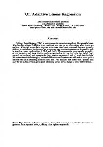
A. Natural Neighbors Natural neighbors are an example of an enclosing neighborhood [26], [27]. The natural neighbors are defined by the Voronoi tessellation V of the training set and test point {X , g}. Given V , the natural neighbors of g are defined to be those training points xj whose Voronoi cells are adjacent to the cell containing g . An example of the natural neighbors is shown in the left diagram of Figure 1. The local coordinates property of the natural neighbors [26] can be used to prove that the natural neighbors form an enclosing neighborhood when g ∈ conv(X ). Though commonly used for 3D interpolation with a specific generalized linear interpolation formula called natural neighbors interpolation, Theorem 1 suggests that natural neighbors may be useful for local linear regression as well. We were unable to find examples where the natural neighbors was used as a neighborhood definition for local regression or nearest neighbor classification. One issue with natural neighbors for general learning tasks is the complexity of computing the Voronoi tessellation of n points in d dimensions is O(n log n) when d < 3 and O((n/d)d/2 ) when d ≥ 3 [28]. B. Natural Neighbors Inclusive The natural neighbors may include a far training sample xi but exclude a nearer sample xj . We propose a variant, natural neighbors inclusive, which consists of the natural neighbors and all training points within the distance to the furthest natural neighbor, maxxj ∈Jg kg − xj k2 . That is, given the set of natural neighbors Jg , the inclusive natural neighbors of g are 

 xj ∈ X kg − xj k2 ≤ max kg − xi k2 . xi ∈Jg

This is equivalent to choosing the smallest k -NN neighborhood that includes the natural neighbors. An example of the natural neighbors inclusive neighborhood is shown in the middle diagram of Figure 1.

(4)

7

C. Enclosing k-NN Neighborhood The linear model in local linear regression may oversmooth if the neighbors are far from the test point g . To reduce this risk, we propose the neighborhood of the k nearest neighbors with the smallest k such that g ∈ conv(Jg (k)), where Jg (k) denotes the k nearest neighbors of g . Note that no such k exists if g 6∈ conv(X ). Therefore, it is helpful to define the concept of a distance to enclosure. Given a test point g and a neighborhood Jg , the distance to enclosure is D(g, Jg ) =

min

z∈conv(Jg )

kg − zk2 .

(5)

Note that D(g, Jg ) = 0 if g ∈ conv(Jg ). Using this definition, the enclosing k-NN neighborhood of g is given by Jg (k ∗ ) where k ∗ = min k

 k D(g, Jg (k)) = D(g, X ) .

If g ∈ conv(X ), this is the smallest k such that g ∈ conv(Jg (k)), while if g 6∈ conv(X ) this is the smallest k such that g is as close as possible to the convex hull of Jg (k). An example of an enclosing k-NN neighborhood is given in the right diagram of Figure 1. An algorithm for computing the enclosing k-NN is given in Appendix B. x9 x8

x9 x8

x1

x2

x4

x8

x1

g

x2

x4

JgNN = {x1 , x2 , x3 , x4 , x6 , x7 }

x2

x4

g

x3 x 5 x7

x6

x1

g

x3 x 5 x7

x9

x3 x 5 x7

x6 JgNN-i = {x1 , . . . , x7 }

x6 JgekNN = {x1 , . . . , x6 }

Fig. 1. In the left figure, the natural neighbors neighborhood JgNN is marked with solid circles. For reference, the Voronoi diagram of this set is dashed. In the center figure the natural neighbors inclusive neighborhood JgNN-i is marked with solid circles; notice that x5 ∈ JgNN-i . The shaded area indicates the inclusion radius maxxj ∈JgNN {kg − xj k2 }. In the right figure, the enclosing k-NN neighborhood JgekNN is marked with solid circles.

8

III. C OLOR M ANAGEMENT Our implementation of printer color management follows the standard calibration and characterization approach described in [6, Section 5]. The architecture is divided into calibration and characterization tables in part to reduce the work needed to maintain the color reproduction accuracy, which may drift due to changes in the ink, substrate, temperature, etc. This empirical approach is based on measuring the way the device transforms device-dependent input colors (i.e. RGB) to printed device-independent colors (i.e. CIELAB). First, n color patches are printed and measured to form the training data X , Y , where X = {xi }i=1:n are the measured CIELAB values and Y = {(yR i , yG i , yB i )}i=1:n are the corresponding RGB values input to the printer. These training pairs are used to learn

the LUTs that form the color management system. The final system is shown in Figure 2: the 3D LUT implements inverse device characterization which is followed by calibration by parallel 1D LUTs that linearize each RGB channel independently.

Fig. 2. A standard color management system: A desired CIELAB color is transformed to an appropriate RGB color that when input to a printer results in a printed patch with approximately the desired CIELAB color.

A. Building the LUTs The three 1D LUTs enact gray-balance calibration, linearizing each RGB channel independently. This enforces that input neutral RGB color values with R=G=B =d will print gray patches (as measured in CIELAB). That is, if one inputs the RGB colors (d, d, d) for d ∈ {0, . . . , 255}, the 1D LUTs will output the RGB values that, when printed, correspond approximately to uniformly-spaced neutral gray steps in CIELAB space. Specifically, for a given neighborhood and regression method, the 918 sample Chromix RGB color chart is printed and measured to form the X , Y training pairs. Next, the L∗ axis of the CIELAB space is sampled with 256 evenly-spaced values GL∗ =



100 255 (i

− 1), 0, 0


i=1:256

to form incremental shades of gray. For each g ∈ GL∗ , a neighborhood Jg is

constructed and three regressions on {yR i | xi ∈ Jg }, {yG i | xi ∈ Jg }, and {yB i | xi ∈ Jg } fit locally linear

9

functions hc :

R3− > R for c = R, G, B. Finally, the 1D LUTs are constructed with the inputs {1, . . . , 256} and

outputs {hc (g) | g ∈ GL∗ }, where c = R, G, B correspond to the three 1D LUTs. The effect of the 1D LUTs on the training data must be taken into account before the 3D LUT can be estimated. The training set is adjusted to find Y 0 that, when input to the 1D LUTs, reproduces the original Y . These adjusted training sample pairs X , Y 0 are then used to estimate the 3D LUT. (Note: in our process all the LUTs are estimated from one printed test chart, as is done in many commercial ICC profile building services. More accurate results are possible by printing a second test chart once the 1D LUTs have been estimated, where the second test chart is sent through the 1D LUTs before being sent to the printer.) The 3D LUT has regularly spaced gridpoints g ∈ GL∗ a∗ b∗ . For the 3D LUTs in our experiment, we used a 17 × 17 × 17 grid that spans the CIELab color space with L∗ ∈ [0, 100] and a∗ , b∗ ∈ [−100, 100]. Previous studies

have shown that a finer sampling than this does not yield a noticeable improvement in accuracy [6]. For each g ∈ GL∗ a∗ b∗ its neighborhood Jg is determined, and regression on {yR 0i | xi ∈ Jg }, {yG 0i | xi ∈ Jg }, and {yB 0i | xi ∈ Jg } fits the locally linear functions hc :

R3− > R for c = R, G, B.

Once estimated, the LUTs can be stored in an ICC profile. This is a standardized color management format, developed by the International Color Consortium (ICC). Input CIELAB colors that are not a gridpoint of the 3D LUT are interpolated. The interpolation technique is not specified in the standard; our experiments used trilinear interpolation [29], a three-dimensional version of the common bilinear interpolation. This interpolation technique is computationally fast, and optimal in that it weights the neighboring grid points as evenly as possible while still solving the linear interpolation equations by choosing the maximum entropy solution to the linear interpolation equations [3, Theorem 2, p. 776].

B. Experimental Setup The different regression methods were tested on three printers: an Epson Stylus Photo 2200 (ink jet) with Epson Matte Heavyweight Paper and Epson inks, an Epson Stylus Photo R300 (ink jet) with Epson Matte Heavyweight Paper and third-party ink from Premium Imaging, and a Ricoh Aficio 1232C (laser engine) with generic laser copy paper. Color measurements of the printed patches were done with a GretagMacbeth Spectrolino spectrophotometer at a 2◦ observer angle with D50 illumination.

10

In our experiments, the calibration and characterization LUTs are estimated using local linear regression and local ridge regression over the enclosing neighborhood methods described in Section II and a baseline neighborhood of 15 nearest neighbors, which is a heuristic known to produce good results for this application [9]. All neighborhoods

are computed by Euclidean distance in the CIELAB colorspace and the regression is made well-posed by adding nearest neighbors if necessary to ensure a minimum of four neighbors. As analyzed in Section V, the enclosing k-NN neighborhood is expected to have roughly seven neighbors, where the word “roughly” is used to capture the fact that the assumptions of Theorem 2 (see Section VA) do not hold in practice. The expected small size of enclosing k-NN neighborhoods led us to also implement a variation of the enclosing k-NN neighborhood which uses a minimum of k = 15 neighbors: this is achieved by adding nearest neighbors to the enclosing k-NN neighborhood if there are fewer than 15. Note that this variant is also an enclosing neighborhood, but ensures smoother regressions than the enclosing k-NN neighborhood. The ridge parameter λ in (2) was fixed at λ = 0.1 for all the experiments. This parameter value was chosen based on a small preliminary experiment, which suggested that values of λ from λ = .001 to λ = 2 would produce similar results. Note that the effect of the regularization parameter is highly nonlinear, and that steeper slopes (higher values of β ) are more strongly affected by the regularization. It is common wisdom that a small amount of regularization can be very helpful in reducing estimation variance, but larger amounts of regularization can cause unwanted bias, resulting in oversmoothing. To compare the color management systems created by each neighborhood and regression method, 729 RGB test color values were drawn randomly and uniformly from the RGB colorspace, printed on each printer, and measured in CIELAB. These measured CIELAB values formed the test samples. This process guaranteed that the CIELAB test samples were in the gamut for each printer, but each printer had a slightly different set of CIELAB test samples. The test samples were then input as the “Desired CIELAB” values to test the accuracy of each estimated LUT, as shown in Figure 2. Each estimated LUT produced estimated RGB values that, when sent to the printer, would ideally yield the test sample CIELAB values. The different estimated RGB values were sent to the printer, printed, ∗ error was computed with respect to the test sample CIELAB values. The measured in CIELAB, and the ∆E94 ∗ error metric is one standard way to measure color management error [6]. ∆E94

11

IV. R ESULTS ∗ error and 95th percentile error for the three printers for each Tables I, III and II show the average ∆E94

neighborhood definition, and each regression method. In addition, we discuss in this section which differences are statistically significantly different as judged at the .05 significance level by Student’s matched-pair t-test. These three metrics (average, 95th percentile, and statistical significance) summarize different aspects of the results, and are complementary in that good performance with respect to one of the three metrics does not necessarily imply good performance with respect to the other two metrics. The baseline is the k = 15 neighbors with local linear regression. Small errors may not be noticeable; though noticeability varies throughout the color space and between ∗ are generally not noticeable. people, errors under 2∆E94

TABLE I ∗ ∆E94 E RRORS FROM THE R ICOH A FICIO 1232C

Neighborhood

Regression

Average Error

95th Percentile Error

Enclosing k-NN

Linear

4.27

8.47

Ridge

3.66

7.38

Linear

4.03

8.30

Ridge

3.45

6.77

Linear

3.74

7.55

Ridge

3.69

7.10

Linear

3.74

7.63

Ridge

4.03

7.70

Linear

4.41

9.84

Ridge

4.16

8.61

Enclosing k-NN Minimum 15 Natural Neighbors Natural Neighbors Inclusive 15 Neighbors

The Ricoh laser printer is the least linear of the three printers, likely due to the printing instabilities that are common with high-speed laser printers. For the Ricoh, all of the enclosing neighborhoods have lower average error and lower 95th percentile error than the baseline of 15 neighbors and linear regression. Further, all of the methods were statistically significantly better than the 15 neighbors baseline, except for enclosing k-NN (linear), which was not statistically significantly different. Changing to ridge regression for 15 neighbors eliminates over 10% of the 95th percentile error. Thus, the adaptive methods and the regularized regression make a clear difference for nonlinear color transformations.

12

TABLE II ∗ ∆E94 E RRORS FROM THE E PSON P HOTO S TYLUS 2200

Neighborhood

Regression

Average Error

95th Percentile Error

Enclosing k-NN

Linear

2.32

5.01

Ridge

2.20

5.03

Linear

2.34

5.00

Ridge

2.32

4.95

Linear

2.40

5.48

Ridge

2.20

5.16

Linear

2.41

5.38

Ridge

2.43

5.61

Linear

2.44

6.52

Ridge

2.43

6.46

Enclosing k-NN Minimum 15 Natural Neighbors Natural Neighbors Inclusive 15 Neighbors

TABLE III ∗ ∆E94 E RRORS FROM THE E PSON P HOTO S TYLUS R300

Neighborhood

Regression

Average Error

95th Percentile Error

Enclosing k-NN

Linear

1.67

3.65

Ridge

1.55

3.32

Linear

1.51

3.05

Ridge

1.52

3.10

Linear

1.71

3.49

Ridge

1.54

2.87

Linear

1.77

3.55

Ridge

1.79

3.55

Linear

1.55

3.32

Ridge

1.55

3.34

Enclosing k-NN Minimum 15 Natural Neighbors Natural Neighbors Inclusive 15 Neighbors

For the Ricoh laser printer, the lowest average error and lowest 95th percentile error are produced by enclosing k-NN minimum 15 (ridge): the 95th percentile error is reduced by 21% over 15 neighbors (ridge), and the total error reduction is 31% over the baseline of 15 neighbors (linear). Enclosing k-NN minimum 15 (ridge) is statistically significantly better than all other methods for this printer. These results suggest that highly nonlinear color transforms can be effectively modeled by local regression using a lower bound on the number of neighbors (to keep estimation variance low) but allowing possibly more neighbors depending on their spatial distribution. On the Epson 2200 all of the enclosing neighborhoods have lower average and 95th percentile error than the

13

baseline of 15 neighbors (linear). However, only enclosing k-NN (ridge), enclosing k-NN minimum 15 (ridge), or natural neighbors (ridge) were statistically significantly better (the other methods were not statistically significantly different). The natural neighbors (ridge) is statistically significantly better than all of the other methods except for enclosing k-NN (linear and ridge), which are not statistically significantly different. Enclosing k-NN (ridge) is statistically significantly better than all of the other methods except for natural neighbors (ridge). These results are consistent with the Ricoh results in that enclosing neighborhoods coupled with ridge regression provide significant benefit. The Epson R300 inkjet fits the locally-linear model well, as evident in the low errors across the board and the small average and 95th percentile error differences between methods. Here, few methods are statistically significantly different, but the natural neighbors inclusive is statistically significantly worse than the other neighborhood methods, including the baseline. We hypothesize that because the natural neighbors inclusive creates in some instances very large neighborhoods, this increase in error may be caused by the bias of oversmoothing. ∗ error because it is considered a more accurate We have presented and discussed our results in terms of the ∆E94 ∗ (Euclidean distance in CIELAB) [6]. In (2) and (1) we minimize error function for color management than ∆E76 ∗ error does the Euclidean error in CIELAB, because this leads to a tractable objective, whereas minimizing ∆E94 ∗ errors were also calculated and compared to the ∆E ∗ errors. The results were very similar in terms not. The ∆E76 94

of the rankings of the regression methods and the statistically significant differences. In summary, the experiments show that using an enclosing neighborhood is an effective alternative to using a fixed neighborhood size. In particular, enclosing k-NN minimum 15 (ridge) achieved the lowest average and 95th percentile error rates for the most nonlinear printer (the laser printer), and was either the best or a top performer throughout. Also, ridge regression showed consistent performance gains over linear regression, especially with smaller neighborhoods. Importantly. the overall low error rates on the inkjet printers suggest that the locally linear model fits sufficiently well on these printers, resulting in less room for improvement over the baseline method.

V. S IZES OF E NCLOSING N EIGHBORHOODS Enclosing neighborhoods adapt the size of the neighborhood to the local spatial distribution of the training and test sample. In this section we consider the key question, “How many neighbors are in the neighborhood?” We

14

consider analytic and experimental answers to this question, and how the neighborhood size will relate to the estimation bias and variance.

A. Analytic Size of Neighborhoods Asymptotically, the expected number of natural neighbors is equal to the expected number of edges of a Delaunay triangulation [27]. A common stochastic spatial model for analyzing Delaunay triangulations is the Poisson point process, which assumes that points are drawn randomly and uniformly such that the average density λ is n points per volume S . Given the Poisson point process model, the expected number of natural neighbors is known for low dimensions: 6 neighbors for two dimensions, 48π 2 /35+2 ≈ 15.5 neighbors for three dimensions, and 340/9 ≈ 37.7 neighbors for four dimensions [27]. The following theorem establishes the expected number of neighbors in the enclosing k-NN neighborhood if the training samples are sampled from a uniform distribution over a hypersphere about the test sample. Theorem 2 (Asymptotic Size of Enclosing k-NN): Suppose n training samples are uniformly sampled from a distribution that is symmetric around a test sample in

Rd. Then, asymptotically as n → ∞, the expected number

of neighbors in the enclosing k-NN neighborhood is 2d + 1. The proof is given in Appendix C. For both the natural neighbors and enclosing k-NN, these analytic results model the training samples as symmetrically distributed about the test point. This is a good model for the general asymptotic case where the number of training samples n → ∞, because if the true distribution of the training samples is smooth then the random sampling of training samples local to the test sample will appear as though drawn from a uniform distribution.

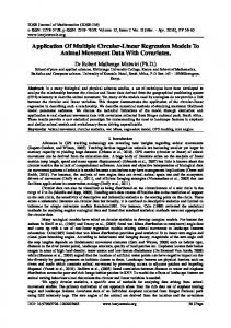
B. Experimental Size of Neighborhoods The analytic neighborhood size results suggest that the natural neighbors is a larger neighborhood on average than the enclosing k-NN neighborhood, which we found to be true experimentally. Representative empirical histograms of the neighborhood sizes are shown in Figure 3. They show the distribution of the neighborhood sizes for the color management of the Ricoh printer from 918 training samples.

15

Fig. 3. 1232C.

Histograms show the frequency of each neighborhood size when estimating the gridpoints of the 3D LUT for the Ricoh Aficio

By design, the enclosing k-NN is the smallest possible k -NN neighborhood that encloses the test point, which should keep estimation bias relatively low because the neighbors are relatively local. The natural neighbors tend to form larger neighborhoods than enclosing k-NN, and a particular natural neighbor could be close or far from the test sample. Thus it is hard to judge how local the natural neighbors are. The natural neighbors inclusive has relatively large neighborhoods, which suggests that some of the natural neighbors must in fact be quite far from the test sample. The large size of the natural neighbors means that the estimated transforms will be fairly linear across the entire colorspace, which can oversmooth the estimation. One cause of large neighborhood sizes is when a test point is outside the convex hull of the entire training set. As discussed in Section I, the set of training samples may not span the full colorspace, resulting in exactly this situation. An illustration of how such cases affect the enclosing neighborhood sizes is provided in Figure 4. Here, the enclosing k-NN neighborhood is {x1 , x2 }. From the Voronoi diagram, one can read that the natural neighbors of g are {x1 , x2 , x3 , x4 , x7 }. The largest of the neighborhoods in this case is the natural neighbors inclusive, composed

of {x1 , x2 , x3 , x4 , x5 , x6 , x7 }. When training and test samples are drawn iid in high-dimensional feature spaces, the test samples tend to be on the boundary of the training set, an effect known as Bellman’s curse of dimensionality [5], [25]. We hypothesize that this effect for high-dimensional feature spaces would cause an abundance of large neighborhoods for the natural neighbors methods.

16

x7

x8

x9

x4 x2 g

x6

x1 x3 x5

Fig. 4.

Example Voronoi diagram for the situation where the test point g lies outside the convex hull of the training samples.

The inclusion of possibly far-away points to “enclose” the test point may result in increased bias. Based on the neighborhood size histograms and our analysis of the different neighborhoods, enclosing k-NN should incur the lowest bias. On the other hand, we expect natural neighbors inclusive to have the largest positive effect on variance because a larger neighborhood tends to lead to lower estimation variance for regression problems, though this matter is not so straightforward for classification.

VI. D ISCUSSION We have proposed the idea of using an enclosing neighborhood for local learning and theoretically motivated it for local linear regression. Such automatically adaptively-sized neighborhoods can be useful in applications where it is difficult to cross-validate a neighborhood size, and in particular we have shown that using enclosing neighborhoods can significantly reduce color management errors. Local learning can have less bias than more global estimation methods, but local estimates can be high-variance [5]. Enclosing neighborhoods limit the estimation variance when the underlying function does have a (noisy) linear trend. Ridge regression is another approach to controlling estimation variance, but does so by penalizing the regression coefficients, which increases bias. In contrast, we hypothesize that the effect of an enclosing neighborhood on bias may be either positive or negative, depending on the actual geometry of the data. It remains an open question how the estimation bias and variance differ between enclosing neighborhoods and the standard k -NN, which uses a fixed, but cross-validated, k for all test samples. The definition of the neighborhood for local learning is important, whether for local regression, or for nearest

17

neighbors classification. We conjecture that using enclosing neighborhoods for other local learning tasks may lead to improved performance, particularly for densely-sampled feature spaces.

ACKNOWLEDGMENTS This work was supported by the Intel GEM fellowship program, the United States Office of Naval Research, the CRA-W DMP, Ricoh and Chromix. We thank Raja Bala, Steve Upton, and Jayson Bowen for helpful discussions.

A PPENDIX A: P ROOF OF T HEOREM 1 Proof: Form the (d + 1)-dimensional vectors g˜ = [g 1]T and a ˜ = [a a0 ]T . Let m = |Jg |, and re-index the training ˜ denote the (d + 1) × m matrix whose ith column is [xi 1]T . samples so that xi ∈ Jg for i = 1, . . . , m. Let X ˜ be the m × 1 vector with Further, let β˜ = [βˆ βˆ0 ]T , let y be the m × 1 vector with ith component f (xi ), and let ω ith component ωi . The least-squares regression coefficients which solve (3) are ˜X ˜ T )−1 Xy ˜ β˜ = (X ˜X ˜ T )−1 X( ˜ X ˜Ta ˜) = (X ˜+ω ˜X ˜ T )−1 X˜ ˜ ω. = a ˜ + (X ˜ =a ˜X ˜ T )−1 XE ˜ [˜ ω ]. Let I denote the m × m identity matrix. Then the covariance matrix of Note that E[β] ˜ + (X

the regression coefficients is ˜ = E cov(β)



 T  T −1 ˜ T −1 ˜ ˜ ˜ ˜ ˜ ˜ ˜ ω] β − a ω] β−a ˜ − (XX ) XE [˜ ˜ − (XX ) XE [˜

˜X ˜ T )−1 X ˜ cov(˜ ˜ T (X ˜X ˜ T )−1 ω) X = (X ˜X ˜ T )−1 X ˜ σ2I X ˜ T (X ˜X ˜ T )−1 = (X ˜X ˜ T )−1 . = σ 2 (X

18

The variance of the estimate yˆ = β˜T g˜ is

  var(ˆ y ) = E (ˆ y − E [ˆ y ])2  h i2  T T ˜ ˜ = E β g˜ − E β g˜ "  #  h i2 T ˜ ˜ = E g˜ β − E β g˜ ˜g = g˜T cov(β)˜ ˜X ˜ T )−1 g˜σ 2 . = g˜T (X

(6)

˜X ˜ T )−1 g˜ ≤ 1 if Jg is an enclosing neighborhood. The proof is finished by showing that g˜T (X

Assume Jg is an enclosing neighborhood. Then by definition it must be that |Jg | ≥ d + 1, and that there exists ˜ = g˜ (which includes the constraint that 1T v = 1) and v  0. The training some weight vector v such that Xv

and test samples are assumed to be drawn iid from a sufficiently nice distribution over the d-dimensional feature space such that the training and test samples are in general position with probability one; that is, the enclosing ˜ is full rank. neighbors and test sample do not lie in a degenerate subspace, and thus it must be that the matrix X  −1 ˜ is well-defined as the m × 1 vector w = X ˜T X ˜X ˜T Then the Moore-Penrose pseudo-inverse of X g˜, and w is ˜ = g˜ such that wT w ≤ v T v for any v that satisfies Xv ˜ = g˜ [30]. the minimum norm solution to Xw

Then,  −1  −1 ˜X ˜T ˜X ˜T X ˜X ˜T wT w = g˜T X X g˜  −1 ˜X ˜T = g˜T X g˜.

(7)

Because 0 ≤ vj ≤ 1 for each j ∈ Jg , it must be that 0 ≤ vj2 ≤ vj . Combining these facts with the property that wT w ≥ 0 because it is a sum of squared (positive) elements, the following holds: 0 ≤ wT w ≤ v T v =

m X j=1

vj2 ≤

m X

vj = 1.

j=1

−1  ˜X ˜T Then from (7) it must also be that g˜T X g˜ ≤ 1, which coupled with (6) completes the proof.

19

A PPENDIX B: M ETHOD FOR C ALCULATING THE E NCLOSING K -NN N EIGHBORHOOD 1) Define an  that is the threshold for how small the distance to enclosure must be before considering the neighborhood to effectively enclose the test point in its convex hull. Generally,  should be small, but how small may depend on the relative scale of the data. For the CIELAB space, where a just noticeable difference is roughly 2∆E , we set  = .1. 2) Re-order the set of training samples {xi } for i = 1, . . . , n by distance from the test point g so that xj is the j th nearest neighbor to g .

3) Add x1 to the set S . 4) Define the indicator function I(xj ), where I(xj ) = 1 if xj lies in the same half-space as g with respect to the hyperplane that passes through x1 and is normal to the vector connecting g to x1 , and I(xj ) = 0 otherwise. 5) Add to the set S the training point x∗j nearest to g in the half-space, that is x∗j = arg min kg − xi k2 xi :I(xi )=1

6) If the distance to enclosure D(g, S) < , then stop iterating, and the set of all training samples closer than x∗j to g form the enclosing k-NN neighborhood.

7) Project g onto the convex hull of S , and denote this point gˆ. Re-define the indicator function I(xj ) = 1 if xj lies in the same half-space as g with respect to the hyperplane that passes through gˆ and is normal to the

vector connecting g to gˆ, and I(xj ) = 0 otherwise. If I(xj ) = 0 for all training samples, then stop iterating, and the set of all training samples that are closer than the farthest member of S form the enclosing k-NN neighborhood. 8) Repeat steps 5-7 until a stopping criteria is met.

A PPENDIX C: P ROOF OF T HEOREM 2 To prove the theorem, the following lemma will be used. Lemma: Given X ∈

Rn×d, let conv(X) denote the convex hull of the rows {xi}i=1:n of X. If and only if the origin

0 ∈ conv(X), then the origin is in the convex hull of some positive scaling of the {xi }i=1:n i.e. , 0 ∈ conv(AX),

20

where A is a positive definite diagonal n × n matrix. Proof of Lemma: Suppose 0 ∈ conv(X). By definition, there exists a weight vector w such that wT 1 = 1, w  0, and wT X = 0}. If X is scaled by the positive definite diagonal matrix A, then it must be shown that there exist a set of weights w0 with the properties that w0T 1 = 1, w0  0, and w0T AX = 0}. Denote the normalization scalar z = wT A−1 1, then it can be seen that one such weight vector that satisfies this condition is w0 = (A−1 w)/z

and we conclude that 0 ∈ conv(AX). Next, suppose that 0 6∈ conv(X), then it must be shown that scaling X by any positive definite diagonal matrix A does not form a convex hull that contains the origin. The proof is by contradiction: assume that 0 ∈ conv(AX) but 0 6∈ conv(X). The first part of this proof could be applied, scaling AX by A−1 , which would lead to the conclusion that 0 ∈ conv(X), thus forming a contradiction.

Now we begin the body of the proof of Theorem 2. Without loss of generality, assume the test point is the origin g = 0. Let X be the random n × d matrix with rows {xi }i=1:n drawn independently and identically from a symmetric distribution in

Rd. Rearrange the rows of X so that they are sorted such that ||xk−1||2 ≤ ||xk ||2 ≤

||xk+1 ||2 for all k . As established in the lemma, without a loss of generality with respect to the event 0 ∈ conv(X),

scale all rows such that ||xj ||2 = 1 for all j . Then 0 ∈ conv(X) if and only if n > d and the row vectors are not all contained in some hemisphere [31]. Let Hn indicate the event that n vectors lie on the same hemisphere, and ¯ n will denote the complement of Hn . Wendel [32] showed that for n points chosen uniformly on a hypersphere H

in

Rd , P(Hn ) = 2−n+1

 d−1  X n−1 k=0

k

∀ n ≥ 1.

(8)

Let Fn be the event that: the first n ordered points enclose the origin, but the first n − 1 ordered points do not

21

enclose the origin. The probability of the event Fn is ¯ n , Hn−1 ) P(Fn ) = P(H ¯ n |Hn−1 )P(Hn−1 ) = P(H = (1 − P(Hn |Hn−1 )) P(Hn−1 ) = P(Hn−1 ) − P(Hn , Hn−1 ) = P(Hn−1 ) − P(Hn ).

(9)

Because one or zero points cannot complete a convex hull around the origin, P(F0 ) = 0 and P(F1 ) = 0. Combining (8) and (9), and using the recurrence relation of the binomial coefficient       n n n+1 + = , k k+1 k+1

= = = = =

 d−1  X n−2

 d−1  X n−1

−2 k k k=0     n−2 n−1 2−n+1 2 − k k k=0      d−1   X n−2 n−2 n−2 −n+1 2 − − 2 k k−1 k k=0             n−2 n−2 n−2 n−2 n−2 n−2 2−n+1 − + − + ... + − d−1 d−2 d−2 d−3 0 −1     n−2 n−2 2−n+1 − d−1 −1   n−2 2−n+1 for all n ≥ 2, d−1

P(Fn ) = 2

−n+2

−n+1

(10)

k=0 d−1  X

where the last line follows because

r −1




= 0 for all r [33, p. 154]. Then,

E[Fa ] =

∞ X a=2

aP(Fa ) =

∞ X a=2

a2

−a+1

  a−2 . d−1

(11)

22

To simplify, change variables to b = a − 2, ∞ X

   b b + 2−b d−1 d−1 b=0      ∞ X b b = +2 2−b−1 b d−1 d−1 b=0 {z } |

E[Fa ] =

b2−b−1



=

b b! 2 b! + (d − 1)!(b − d + 1)! (d − 1)!(b − d + 1)!

=

(b + 1) b! b! + (d − 1)!(b − d + 1)! (d − 1)!(b − d + 1)!

d (b + 1)! b! + d!(b − d + 1)! (d − 1)!(b − d + 1)!      b+1 b = d + d d−1       b+1 b+1 b =d + − d d d      ∞ X b+1 b = 2−b−1 (d + 1) − , d d =

b=0

where the second to last line follows from (10). Expand the recurrence,         1 2 −1 0 −2 −2 1 E[Fa ] = lim 2 (d + 1) −2 + 2 (d + 1) −2 + ... n→∞ d d d d         n n−1 n+1 n +2−n (d + 1) − 2−n + 2−n−1 (d + 1) − 2−n−1 d d d d       
n
1 −n−1 −2 −1 0 + ... + 2 2(d + 1) − 1 + 2 2(d + 1) − 1 = lim 2 n→∞ d d d   n+1 +2−n−1 (d + 1) d    !  ! n X i n+1 −1 0 −i−1 −n−1 = lim 2 + 2 (2d + 1) +2 (d + 1) . n→∞ d d d 

−1

i=1

The first and third terms in this equation converge to zero as n → ∞, leaving E[Fa ] = (2d + 1)

∞ X i=1

2

−i−1

  i . d

23

Using the identity

0 d




= 0 [33, p. 155], and the summation [33, p. 199] ∞   X zd i i = z d (1 − z)d+1 i=0

with z = 1/2, establishes the result: E[Fa ] = 2d + 1.

R EFERENCES [1] W. Lam, C. Keung, and D. Liu, “Discovering useful concept prototypes for classification based on filtering and abstraction,” IEEE Trans. on Pattern Analysis and Machine Intelligence, vol. 24, no. 8, pp. 1075–1090, August 2002. [2] R. C. Holte, “Very simple classification rules perform well on most commonly used data sets,” Machine Learning, vol. 11, pp. 63–90, 1993. [3] M. R. Gupta, R. Gray, and R. Olshen, “Nonparametric supervised learning by linear interpolation with maximum entropy,” IEEE Trans. on Pattern Analysis and Machine Intelligence, vol. 28, no. 5, pp. 766–781, May 2006. [4] C. Loader, Local Regression and Likelihood.

New York: Springer, 1999.

[5] T. Hastie, R. Tibshirani, and J. Friedman, The Elements of Statistical Learning. [6] R. Bala, Digital Color Handbook. [7] P. Emmel, Digital Color Handbook.

New York: Springer-Verlag, 2001.

CRC Press, 2003, ch. 5: Device Characterization, pp. 269–384. CRC Press, 2003, ch. 3: Physical Models for Color Prediction, pp. 173–238.

[8] B. Fraser, C. Murphy, and F. Bunting, Real World Color Management.

Berkeley, CA: Peachpit Press, 2003.

[9] M. R. Gupta and R. Bala, “Personal communication with Raja Bala,” June 21 2006. [10] A. E. Hoerl and R. Kennard, “Ridge regression: biased estimation for nonorthogonal problems,” Technometrics, vol. 12, pp. 55–67, 1970. [11] K. Fukunaga and L. Hostetler, “Optimization of k-nearest neighbor density estimates,” IEEE Trans. on Information Theory, vol. 19, pp. 320–326, 1973. [12] R. Short and K. Fukunaga, “The optimal distance measure for nearest neighbor classification,” IEEE Trans. on Information Theory, vol. 27, no. 5, pp. 622–627, 1981. [13] K. Fukunaga and T. Flick, “An optimal global nearest neighbor metric,” IEEE Trans. on Pattern Analysis and Machine Intelligence, vol. 6, pp. 314–318, 1984. [14] J. Myles and D. Hand, “The multi-class metric problem in nearest neighbour discrimination rules,” Pattern Recognition, vol. 23, pp. 1291–1297, 1990. [15] J. Friedman, “Flexible metric nearest neighbor classification,” Technical Report, Stanford University, CA, 1994. [16] C. Domeniconi, J. Peng, and D. Gunopulos, “Locally adaptive metric nearest neighbor classification,” IEEE Trans. on Pattern Analysis and Machine Intelligence, vol. 24, no. 9, pp. 1281–1285, 2002.

24

[17] R. Paredes and E. Vidal, “Learning weighted metrics to minimize nearest-neighbor classification error,” IEEE Trans. on Pattern Analysis and Machine Intelligence, vol. 28, no. 7, pp. 1100–1110, 2006. [18] T. Hastie and R. Tibshirani, “Discriminative adaptive nearest neighbour classification,” IEEE Trans. on Pattern Analysis and Machine Intelligence, vol. 18, no. 6, pp. 607–615, 1996. [19] D. Wettschereck, D. W. Aha, and T. Mohri, “A review and empirical evaluation of feature weighting methods for a class of lazy learning algorithms,” Artificial Intelligence Review, vol. 11, pp. 273–314, 1997. [20] J. Peng, D. R. Heisterkamp, and H. K. Dai, “Adaptive quasiconformal kernel nearest neighbor classification,” IEEE Trans. on Pattern Analysis and Machine Intelligence, vol. 26, pp. 656–661, 2004. [21] R. Nock, M. Sebban, and D. Bernard, “A simple locally adaptive nearest neighbor rule with application to pollution forecasting,” Intl. Journal of Pattern Recognition and Artificial Intelligence, vol. 17, no. 8, pp. 1–14, 2003. [22] J. Zhang, Y.-S. Yim, and J. Yang, “Intelligent selection of instances for prediction functions in lazy learning algorithms,” Artificial Intelligence Review, vol. 11, pp. 175–191, 1997. [23] B. Bhattacharya, K. Mukherjee, and G. Toussaint, “Geometric decision rules for instance-based learning,” Lecture Notes Computer Science, pp. 60–69, 2005. [24] L. Devroye, L. Gyorfi, and G. Lugosi, A Probabilistic Theory of Pattern Recognition.

New York: Springer-Verlag Inc., 1996.

[25] P. Hall, J. S. Marron, and A. Neeman, “Geometric representation of high dimension, low sample size data,” Journal Royal Statistical Society B, vol. 67, pp. 427–444, 2005. [26] R. Sibson, Interpreting multivariate data.

John Wiley, 1981, ch. A brief description of natural neighbour interpolation, pp. 21–36.

[27] A. Okabe, B. Boots, K. Sugihara, and S. Chiu, Spatial Tessellations.

Chichester, England: John Wiley and Sons, Ltd., 2000, ch. 6,

pp. 418–421. [28] C. B. Barber, D. P. Dobkin, and H. Huhdanpaa, “The quickhull algorithm for convex hulls,” ACM Trans. Math. Softw., vol. 22, no. 4, pp. 469–483, 1996. [29] H. Kang, Color Technology for Electronic Imaging Devices. [30] S. Boyd and L. Vandenberghe, Convex Optimization.

United States of America: SPIE Press, 1997.

Cambridge, UK: Cambridge University Press, 2006.

[31] R. Howard and P. Sisson, “Capturing the origin with random points: Generalizations of a Putnam problem,” College Mathematics Journal, vol. 27, no. 3, pp. 186–192, May 1996. [32] J. Wendel, “A problem in geometric probability,” Math. Scand., vol. 11, pp. 109–111, 1962. [33] R. L. Graham, D. E. Knuth, and O. Patashnik, Concrete Mathematics.

New York: Addison-Wesley, 1989.