surface (Singh & Bhallamudi 1998). In particular, the hydraulic description of the overland flow is very important for flood risk assessment because it allows the ...
European Water 38: 13-23, 2012. © 2012 E.W. Publications
Two-dimensional model for overland flow simulations: A case study P. Costabile1, C. Costanzo1, F. Macchione1 and P. Mercogliano2,3 1
LAMPIT, LAboratorio di Modellistica numerica per la Protezione Idraulica del Territorio, Dipartimento di Difesa del Suolo, University of Calabria, Italy 2 Meteo System & Instrumentation CIRA (Italian Aerospace Research Centre), Capua, Italy 3 Impact on Soil and Coast Division CMCC (EuroMediterranean Centre for Climate Change), Lecce, Italy
Abstract:
This paper deals with the problem of flood generation and propagation at catchment scale. The main aspect of the work is the use of 2D fully dynamic shallow water equations as tool of analysis for spatial and temporal overland flow evolution starting from an observed or predicted rain input. The paper firstly focuses on the model description. The governing equations and the numerical integration scheme are presented. Then some aspects related to the robustness of the numerical model are discussed providing three techniques able to improve its stability in presence of very shallow water depths over complex topographies. After recalled the main features of the meteorological model used in the paper, attention is focused on the simulation of a real event occurred in a small basin in Italy whose drainage area is around 40 km2. Two simulations are presented in which observed and simulated rainfall have been used, respectively, as input of the overland flow model. The overall result is satisfactory.
Keywords:
overland flow, shallow water equations, meteorological models
1. INTRODUCTION Many problems of flood routing, river management and civil protection consist of evaluation of the maximum water levels and discharges that may be attained at particular locations during a meteorological event. The hydraulic features of overland flow are significantly related to the characteristics and spatial variability of rainfall. In particular, convective rainstorm events often induce extreme floods, known as flash floods, that are one of the most destructive natural hazards in the Mediterranean region. Runoff is dependent not only by precipitation but also it is influenced by soil and topography conditions. Indeed surface runoff is a dynamic part of the response of a watershed to the rainfall; it is known to cause surface erosion and it is quite often associated to a sudden rise of the stream hydrograph. So the use of numerical modeling seems to be necessary for both predicting the flood-prone areas and, consequently, planning the damage minimization policies. The use of an accurate model is very important to manage the risk associated with potential extreme meteorological events at basin scale. Several methods exist, accepted as standard procedures, that are able to model the rainfall-runoff process. The level of model sophistication depends on the assumptions made for simplifying the governing equations before they are solved. The complexity varying from the linear lumped black box models to non linear physically based distributed models (Taskinen and Bruen 2007). Indeed the mathematical modeling of overland flow is very complex because it involves the description of several phenomena such as the surface flow and groundwater flow with seepage at the ground surface (Singh & Bhallamudi 1998). In particular, the hydraulic description of the overland flow is very important for flood risk assessment because it allows the computation of flow depths and velocities. Overland flow with rainfall as source of lateral inflow can be treated as an unsteady and shallow flow which occurs in natural watershed and also in urban drainage areas. A strong effort has been made in the literature for modeling these situations leading to a number of numerical models based on different levels of detail according to the simplifications introduced to describe the hydraulic processes. The most powerful approach to deal with these situations is represented by 2D
14
P. Costabile et al.
shallow water equations because of their capacity to simulate a number of complex phenomena that occur in real topography such as backwater effects and transcritical flow. The work of Zhang & Cundy (1989) represents one of the first attempts to model overland flow using the fully 2D shallow water equations; the authors used a finite difference scheme to solve them. Esteves et al. (2000) and Fiedler & Ramirez (2000) developed numerical models that couple the surface flow and infiltration process considering the variations in the topographic elevation and in the soil hydraulics parameters. The problems of instabilities and convergence due to highly non linear nature of the governing equations limited, in the past, the use of the complete shallow water equations. Indeed a number of numerical problems exist in the use of the 2D unsteady flow modeling for the propagation of a surface runoff in complex topography; these are mainly due to small water depths over high slope, adverse slope and irregular topography. For example Ajayi et al. (2008) proposed a model to simulate hortonian overland flow in which, within a numerical model based on the leapfrog scheme for the integration of 2D shallow water equations, a time filtering is introduced to ensure smooth results in consecutive time steps. Unami et al. (2009) used the 2D complete unsteady flow equations, solved with a finite volume method, to study the runoff processes in Ghanaian inland valleys during flood events; in their model particular attention is paid to achieve stable computation in complex topographies. Heng et al. (2009) proposed a numerical model to describe the overland flow and the associated soil erosion phenomena; the numerical scheme, based on a MUSCLHancock method, minimizes the spurious oscillation that may arise from both the numerical imbalance between source terms and flux gradient and the treatment of wet-dry fronts with very shallow flows. The main purpose of this paper concerns the development and testing of an overland flow model based on the 2D shallow water equations able to provide accurate, efficient and robust predictions for flood hazard assessment at basin scale. In particular the governing equations of the overland flow model together with the numerical scheme used to their numerical integration are firstly presented. A brief section is also provided in which the influence of some numerical techniques on the model stability is discussed. Prior to focus attention on model performances, the main features of the meteorological model used in the paper are presented. Finally, two simulations are presented in which observed and simulated rainfall have been used, respectively, as input of the overland flow model.
2. OVERLAND FLOW MODEL As already stated, the 2D fully dynamic shallow water equations have been used in this paper. Rain contribution and infiltration losses are considered as source terms in the mass continuity equation. So the governing equations are the following: ∂U ∂ F ∂G + + =S ∂t ∂x ∂ y
(1)
where: ⎛ ⎞ r− f hu ⎛ ⎞ ⎛ ⎞ hv ⎛ h⎞ ⎜ ⎟ ⎜ ⎟ ⎜ ⎟ ⎜ ⎟ ⎜ gh ( S0 x − S fx ) ⎟ huv ; = U = ⎜ hu ⎟ ; F = ⎜ hu 2 + gh 2 / 2 ⎟ ; G = ⎜ S ⎟ ⎜ ⎟ ⎜ hv ⎟ 2 2 ⎜ ⎟ ⎜ ⎟ huv ⎜ gh ( S0 y − S fy ) ⎟ ⎝ ⎠ ⎝ hv + gh / 2 ⎠ ⎝ ⎠ ⎝ ⎠
(2; 3; 4; 5)
in which: t is time; x, y are the horizontal coordinates; h is the water depth; u, v are the depthaveraged flow velocity in x- and y- directions; g is the gravitational acceleration; S0x, S0y are the
European Water 38 (2012)
15
bed slopes in x- and y- directions; Sfx, Sfy are the friction slopes in x- and y- directions, which can be calculated from Strickler’s formula; r is the rain intensity and f are the infiltration losses. In the literature the use of models based on the kinematic or diffusive wave approximation is quite common. The choice of the fully dynamic model has been consequent to an in-depth analysis and a comparative survey on the performances of overland flow models. In particular in Costabile et al. (2011) models based on fully dynamic, diffusive and kinematic wave properties have been developed, tested and validated using numerical tests commonly used in the literature. From that analysis it was deduced that the use of simplified models may lead to important errors in situations characterized by impulsive phenomena over complex topographies.
3. NUMERICAL INTEGRATION SCHEME The finite volume method has been used to the numerical integration of the governing equations. It considers the integral form of the shallow water equations which facilitate the implementation of shock capturing schemes on different mesh types. The system of equations is integrated over an arbitrary control volume Ωi,j and, in order to obtain surface integrals, the Green theorem has been applied to each component of the flux vectors (for example F and G) leading to: ∂ ∂t
∫
Ud Ω +
Ωi , j
v∫ [F, G ] ⋅ n dL = ∫
∂Ω i , j
Sd Ω
(6)
Ωi , j
where ∂Ωi,j is the boundary enclosing Ωi,j, n is the unit vector normal and dL is the length of each boundary. Denoting by Ui,j the average value of the flow variables over the control volume Ωi,j at a given time, the equation (6) may be discretized as: U in,+j1 = U in, j −
Δt Ωi, j
4
∑ [F, G ] r =1
r
⋅ n r ΔLr + ΔtS in, j
(7)
Several algorithms have been proposed for the flux vector computation and comparative surveys on the performances of several first and second order upwind and central numerical schemes were presented in previous works (see for instance Macchione & Morelli 2003, Costanzo & Macchione 2005). In what follows the LHLL first order upwind scheme has been implemented and used for integrating the complete model (Fraccarollo et al. 2003). LHLL is a finite-volume Godunov-type one and is based on a HLL scheme for the homogeneous conservative-part of the system, and on a discretization of the non-conservative term with a "lateralization". It gives two values for the numerical fluxes, the first one for the right side of the intercell (R), the second one for the left side (L), with the following expression: FLLHLL = F HLL − ,R
sL , R sL − sR
gh� ( z R − z L )
(8)
where L and R are, respectively, the left and the right initial values of Riemann’s problem; FHLL refers to an HLL evaluation of the fluxes (Harten et al.,1983): ⎧[FL ⎪ ⎪s F ⋅n −s F ⋅n +s s ( U −U ) FHLL = ⎨ R L r L R r L R R L sR −sL ⎪ ⎪FR ⎩
if sL ≥0 if sL ≤0≤ sR if sR ≤0
(9)
16
P. Costabile et al.
sL and sR are the expressions of the wave celerities calculated as in Toro (2001), zL and zR are the bed elevations, and: h� = 0.5 ( h R + h L )
(10)
3.1 Numerical techniques for preventing instability problems It is well-known in the literature that the presence of small depths over complex topography and wet-dry interfaces may lead to several numerical problems when using fully dynamic wave equations. In overland flow simulations these problems clearly are amplified by the presence of a great number of computational dry cells that become wet because of the rainfall input and subsequently dry out due to high bed slopes. The influence of some numerical techniques has been analyzed in Costabile et al. (2010) in order to evaluate the improvements induced on the solution in simulating the surface runoff over a complex topography. In particular, three kind of controls have been implemented in the LHLL scheme that improve the stability of the numerical model. The first one deals with the interface between dry and wet cells. Let's consider a wet cell next to a dry cell on the right where hL>0, hR=0 and the surface water level HR>HL; in this case, without any modification, a non physical flux will be necessarily computed across the common interface. So a temporary modification of the right cell bed level has to be introduced to avoid this spurious flux and the wet cell velocity component normal to the wet-dry cell interface is set to zero to ensure the no flow condition (Burguete et al. 2004; Liang & Borthwick 2009). Another source of errors and instabilities comes from steep bed slopes: in particular, more water than that actually contained in the wet cell may be computed as flowing in the dry cell and, as a consequence, the negative water depth will induce numerical instability; in this case a number of modifications have to be introduced in the scheme to prevent the code failure. First of all, a minimum water depth hs has to be considered and, when a lower value is computed, the cell is considered dry with the velocity components set to zero and the cell itself is filled up to hs. Then, to ensure the mass conservation, water is subtracted from the adjacent cell containing most water and, in the same cell, the variables hu and hv are also modified in such a way to maintain u and v the same as before. The last numerical technique concerns the spurious effects induced by the friction slope. Singularities may arise due to the bed friction term when the water depth becomes very small as it is often present in overland flow simulations: for small water depths, the bed friction term dominates over other terms in the momentum equation, as the term h4/3 appears in the denominator. The most common and simple procedure is the pointwise discretization of the terms independent of the methodology used for the rest of the system. However this criterion in presence of high friction or low water depth leads to numerical instabilities. Therefore an implicit or semi-implicit treatment of the friction source term has been used.
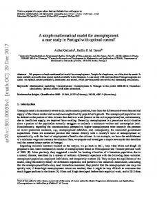
4. METEOROLOGICAL MODELS Two different kinds of numerical weather prediction models were used to perform the simulations: the global model and the regional model (figure 1). The selected atmospherical global model is the Integrated Forecast system (IFS) developed by ECMWF (ECMWF 2004) and described in details by Simmons et al. (1989). It is a global model producing atmospheric forecast on the whole globe with a horizontal resolution of about 16 km and with a forecast time range up to 10 days. The model is constituted by six equations governing the primitive equation atmospheric model (Holton 2004).The first two are the gas law and the hydrostatic equation; they are diagnostic and concern the relation among different parameters. The other four equations are prognostic and describe the changes with time of the horizontal wind components, temperature and water vapour content of an air parcel, and of the surface pressure and are the equation of continuity, the equation
European Water 38 (2012)
17
of motion, the thermodynamic equation and the conservation equation for moisture (Persson 2001). This model is employed to forecast the synoptic phenomena on the world, as extratropical and tropical cyclones, fronts, jet streams and baroclinic waves. For this reason, regional or limited area models should be used to provide forecast on a smaller area than global model but with a higher spatial (from 1 to 10 km) and temporal resolution. These models allow a more accurate parameterization of the physical processes and in particular they solve the processes at meso γ and meso β scale as thunderstorms, squall lines, supercells, mesoscale convective complexes (Holton 2004). Currently, the mesoscale models are the best ones able to assess some high-impact events such as small hurricanes, storms and very extensive tornadoes. Due to the high spatial resolution they can run only on a limited area and, then, they need to be initialized by global models through proper initial and boundary condition. Regional models represent a dynamic downscaling of the global models. In this application the global model IFS is coupled to the limited area model COSMO-LM, developed by COSMO Consortium (Doms & Schattler 1998). COSMO-LM model is a non hydrostatic limited area atmospheric prediction model; it is based on the primitive thermohydrodynamical equations describing compressible flow in a moist atmosphere. The model equations are formulated in rotated geographical coordinates and a generalized terrain following height coordinate. A variety of physical processes are taken into account by parameterization scheme (grid scale cloud and precipitation, moist convection, radiation, soil model, surface layer and subgrid- scale turbulence). The prognostic variables of the model are horizontal and vertical Cartesian wind components, pressure perturbation, temperature, specific humidity, cloud water content and optionally cloud ice content, turbulent kinetic energy, specific water content of rain and snow (Doms 2002).
Figure 1. Atmospherical simulation models flow charts
Currently two model versions are available: the first with a horizontal resolution of 7 km and a temporal forecast range up to 72 hours and a second one with 2.8 km of horizontal resolution and a forecast range up to 24 hours. It is expected that the latter will allow a direct simulation of severe weather events triggered by deep moist convection, such as supercell thunderstorms, intense mesoscale convective complexes, prefrontal squall lines storm (Trentmann et al. 2009). Different simulations have been performed using COSMO LM 7 km and 2.8 km. Initial and boundary data are taken from ECMWF forecasts data (with about 40 km of horizontal resolution). The simulations are initialized at 00 UTC with a forecast time range of 24 hours. The Tiedtke scheme for sub grid scale convection (Tiedtke 1989) is used for the simulation at 7 km while for the simulation at 2.8 km have been used two different configurations. The first one is called "shallow convection" in which the deep convection is evaluated explicitly, due to the high resolution, and only a parameterization for the shallow convection is used. The second one is called "all convection" in which the deep, mid level and shallow convection are parameterized in the same way than the configuration at 7 km. The convection scheme fulfils several objectives. Apart from computing the cloud production it also computes the convective precipitation, the vertical transport
18
P. Costabile et al.
of moisture and momentum, and the temperature changes due to release of latent heat (heating) or evaporation (cooling). Shallow convection is associated with clouds with limited vertical development and involves the growth of small droplets by condensation while deep convection is associated with clouds with very high vertical development and intense and localized rain phenomena. Either versions of COSMO-LM (7 km or 2.8 km) can be used to initialize the model for flash flood prediction but only the prediction resulting from COSMO LM 2.8 km shallow convection is used for the overland flow simulation shown in this paper.
5. MODEL APPLICATION: HYDRAULIC SIMULATION OF A REAL FLOOD EVENT Predictive ability and adequacy of the implemented hydraulic model have been tested by applying it on a sub basin of Reno River (Italy) to simulate the flood event occurred on 7th-9th November 2003. 5.1 Description of the watershed The watershed is located in the most upstream part of Reno River basin (Italy), at the closure section of Pracchia, in the Tuscan part of the Reno basin, and near the Emilia Romagna Region, North Italy. The drainage area is around 40 km2. The average elevation is of 913 m above sea level, the highest peak and the outlet being at an altitude of 1634 and 1610 m above sea level respectively. The hillslopes are significantly steep, with 47% of the area having slopes over 20°. A Digital Elevation Model (DEM) with 20 m cell size has been generated from the topographical maps (figure 2). The spatially-distributed description of the soil use on the watershed comes from the CORINE Land Cover database. In figure 3 CORINE land cover classes on the watershed are shown. The vegetation cover is constituted primarily by broad-leaved (almost 77%) and mixed/coniferous (15%) forests. In the middle part of the basin, there are urbanized (4%), industrial areas (1%) and pastures (1%). A small part of the basin (2%) is cultivated.
Figure 2. Digital Elevation Model (20 m x 20 m)
European Water 38 (2012)
19
Figure 3. Spatially – distributed description of the soil use on the watershed (CORINE)
5.2 Computation of the net rainfall In order to exploit fully the advantages of the spatially variable representation of the rainfallrunoff transformation processes, it is necessary a reliable assessment of the spatial distribution of both the total (gross) rainfall fields and of the part that actually becomes surface runoff (net rainfall). These evaluations were carried out by Brath et al. (2009). Ground precipitation data are available in the form of the observed hourly rainfall depths that were measured in each one of the nine raingauges located within or close to the catchment. On the basis of such point data, for each hour, a rainfall field, spatially-distributed over the entire watershed area was estimated. At each hourly time step of the event, the rainfall in correspondence of each 20 m x 20 m cell is estimated with an inverse squared distance weighting of the raingauges observations. The mean area gross precipitation accumulated over each hour of the event is depicted in the figure 4. The net rain fields used as input in the overland flow model were also obtained by Brath et al. (2009). In that report it was assumed that the flood event may be appropriately modeled by an approach that is primarily driven by a Hortonian (infiltration excess) surface runoff generation mechanism. The hydrological analysis is based on a rather classical, simplified approach that represents the spatial distribution of excess precipitation with a single parameter, the runoff coefficient. In particular, following the approach proposed in the WetSpa distributed rainfall-runoff model (Wang et al., 1996; De Smedt et al., 2002), the surface runoff or rainfall excess for each raster cell was calculated by Brath et al. (2009) using a moisture-related modified rational method in relation with a potential runoff coefficient C. The maps of land use and soil type were used to infer a first estimate of the values of the only one spatially-varied parameter, that is the potential runoff coefficient. Then a calibration procedure was performed in that report by applying scalar multipliers or additive constants to parameter maps until the desired match between simulated and observed data is obtained. The value of such correction factor is derived from the observed hydrograph, or better from its separation in surface and base flows. Further details may be found in Brath et al. (2009).
20
P. Costabile et al.
Mean Areal Precipitation (mm)
25 20 15 10 5 0 1 4 7 10 13 16 19 22 25 28 31 34 37 40 43 46 49 52 55 58 61 64 67 70 Hours (from 7 november 2003, 0:00) Figure 4. Mean area gross precipitation over the watershed (after Brath et al. 2009)
5.3 Simulation of the event The flood event occurred from 7 to 9 November 2003 was characterized by significant rainfall intensities. For validation purposes, the observed water levels recorded at 30 minutes time intervals at Pracchia cross-section, transformed in the discharge hydrograph using a properly rating curve (Brath et al. 2009), were also used. In this section, the simulations carried out using the overland flow model initialized by the net rainfall fields obtained by Brath et al. (2009) are presented and discussed. The Strickler coefficient was assumed variable in space according to land cover as suggested in the literature (Mahmood and Yevjevich, 1975, Chow et al., 1988, Julien, 2002). No calibration procedure has been performed to determine the Strickler coefficient values despite they can be considered a sort of calibration parameters for the hydraulic propagation models (Aronica et al. 2002, Bates 2004). In particular assuming the Strickler’s roughness coefficient for forest equal to 15 m1/3/s, for discontinuous urban fabric and industrial or commercial units equal to 20 m1/3/s and for channel cells equal to 35 m1/3/s, the numerical results are in good agreement with the observed discharge hydrograph at the outlet station shown in figure 5. In particular the computed peak discharge, time to peak discharge and run off volume are very close to the corresponding observed values. However, despite the shape of the computed hydrograph is similar to the observed one, the numerical model shows in the first part of the rising limb of the hydrograph an overestimation of the discharges. Probably this overestimation is due to the infiltration model that could have underestimated the infiltration ratio. However, considering that in the calibration of the model the formation of the surface runoff and its propagation have been carried out separately in a decoupled way, it is believed that the achievements are more than satisfactory. It is important to observe that the use of the numerical techniques discussed in section 4 played an important role on the stability of the model especially at the early stage of the phenomenon in which very small rainfall intensities, and consequently very small hydraulic depths, occurred.
European Water 38 (2012)
21
Figure 5. Comparison between observed and simulated runoff hydrograph at Pracchia station from 00:00 (8th November 2003)
6. COUPLING WEATHER FORECAST AND OVERLAND FLOW MODEL After the validation showed in the previous section, the overland flow model has been used also to simulate the same flood event starting from rainfall data simulated by the COSMO-LM 2.8 km model with the configuration called “shallow convection”. The mesh size of the meteorological model is coarser than that used in the propagation model so a spatial interpolation of the rainfall data on the finer mesh used in the hydraulic model is needed. Indeed, since this is not the purpose of the paper, for the sake of simplicity a constant rain intensity value was considered for all the computational cells of the hydraulic model that "fall" on a computational cell of the meteorological model.
Figure 6. Comparison between observed and simulated runoff hydrograph at Pracchia station from 00:00 (8th November 2003)
22
P. Costabile et al.
The net rainfalls, that are the input of the overland flow model, have been computed using the same run-off coefficients used in the calibration phase. In the figure 6 the comparison between the observed and simulated hydrograph is shown. The overall result obtained by the coupling between weather forecast and overland flow model is quite encouraging. In particular the discharge peak value is very similar to the observed one even if the time to peak is a little overestimated. Though the simulated hydrographs reproduces the overall shape of the observed one, it should be noted that a significant overestimation of the discharge values occur in the first hours of the simulation. This is clearly due to an overestimation of the predicted rainfall volume.
7. CONCLUSIONS In this paper a numerical model for overland flow simulation water equations has been presented. In particular, the model is based on the 2D shallow water equations in which the rainfall input and infiltration losses are considered as a source term in the mass continuity equation. The governing equations have been numerically integrated using a finite volume scheme whose stability is further favored by introducing specific techniques in order to avoid numerical sources of errors that could lead to spurious oscillations and failure of the simulations. The overland flow model has been used to study a real event on a sub-basin located on the upper part of the Reno basin (north Italy). Two simulations have been shown in the paper. In the first one, the observed net rainfalls, as computed in Brath et al. (2009), were used as input of the overland flow model. In this case, the numerical results highlight a reasonably good agreement between observed and simulated hydrographs in terms of discharge peak value, time to peak and shape of the hydrographs. In the second application, the overland flow model has been initialized by the rainfall fields predicted by using the COSMO-LM 2.8 km that is a non hydrostatic limited area atmospheric prediction model. The overall result obtained by the coupling between weather forecast and overland flow model is quite encouraging since the shape of the hydrograph and the discharge peak value are very similar to the observed one.
ACKNOWLEDGMENTS This paper is the result of a research work between LAMPIT and CMCC (Centro Euro Mediterraneo per i Cambiamenti Climatici, Euro – Mediterranean Centre for Climate Change). In particular this research was supported in part by the funding project “Modellistica idraulica delle alluvioni conseguenti ad eventi meteorologici intensi” (Numerical modelling of floods due to heavy rainfalls) in the framework of the project “Centro Euro Mediterraneo per I Cambiamenti Climatici: creazione di un centro di respiro internazionale per la ricerca nel campo dei cambiamenti climatici”.
REFERENCES Ajayi, A. E., van de Giesen, N. & Vlek, P. (2008). "A numerical model for simulating Hortonian overland flow on tropical hillslopes with vegetation elements". Hydrol. Processes, 22: 1107-1118. Aronica, G., Bates, P. D. & Horritt, M. S. (2002).”Assessing the uncertainty in distributed model predictions using observed binary pattern information within GLUE". Hydrol. Processes, 16, 2001–2016. Bates, P. D. (2004). “Remote sensing and flood inundation modelling”. Hydrol. Processes, 18, 2593–2597. Brath, A., Toth, E. & Domeneghetti, A. (2009). " Processing and hydrological analysis of the data of the November 2003 flood event in the Reno River closed at Pracchia". CMCC Research paper RP-0107, available on http://www.cmcc.it/publicationsmeetings/publications/research-papers. Brufau P., García Navarro P. & Vazquez-Cendon M. E. (2004). “Zero mass error using unsteady wetting–drying conditions in shallow flows over dry irregular topography”. Int. J. Numer. Methods Fluids, 45:1047–1082. Burguete J., Garcìa-Navarro P., Murillo J. (2008). “Friction term discretization and limitation to preserve stability and conservation in the 1D shallow-water model: Application to unsteady irrigation and river flow". Int. J. Numer. Methods Fluids, 58: 403– 425.
European Water 38 (2012)
23
Costabile, P., Costanzo, C. & Macchione, F. (2010). "Numerical aspects in simulating overland flow events". Proocedings of the First IAHR European Congress, May 2010, Edinburgh, Scotland. Costabile, P., Costanzo, C. & Macchione, F. (2011). "Overland flow hydraulic simulation using two-dimensional finite volume scheme". J. Hydroinf., doi:10.2166/hydro.2011.077. Costanzo, C., Macchione, F. (2005). "Comparison of two-dimensional finite volume schemes for dam break problem on an irregular geometry”. Proc. of the XXXI IAHR Congress, Seoul, Korea, Theme D, 3372-3381. Chow,V.T., Maidment, D.R., Mays, L.W, (eds.). (1988). Applied Hydrology, McGraw-Hill International Editions, New York. Doms, G. (2002). “The LM cloud ice scheme”. Cosmo Newsletter, No. 2, 128-136. Available on line at www.cosmo-model.org. Doms, G., Schattler, U. (2003). "A description of the Nonhydrostatic Regional Model LM, Part 1- Dynamics and numerics". available at www.cosmo-model.org. ECMWF (2004). "Part VII: ECMWF Wave-model documentation, in IFS documentation CY28r1", available at http://www.ecmwf.int/research/ifsdocs/CY28r1/index.html. Esteves, M., Faucher, X., Galle, S. & Vauclin, M. (2000). "Overland flow and infiltration modelling for small plots unsteady rain: numerical results versus observed values". J. Hydrol., 228: 265-282. Fiedler, F. R., Ramirez, J. A. (2000). "A numerical method for simulating discontinuos shallow flow over an infiltrating surface". Int. J. Numer. Methods Fluids, 32: 219-240. Fraccarollo, L., Capart, H., & Zech, Y. (2003). "A Godunov method for the computation of erosional shallow water transient." Int. J. Numer. Methods Fluids, 41: 951–976. Heng, B. C. P, Sander, G. C., Scott, C. F. (2009). "Modeling overland flow and soil erosion on nonuniform hillslopes: a finite volume scheme". Water Resour. Res., 45, W05423. Holton, J.R. (2004). An introduction to Dynamic Meteorology, Elsevier Academic Press. Julien P. Y. (2002). River Mechanics. Cambridge University Press (UK). Liang, Q., Borthwick A. G.L. (2009). “Adaptive quadtree simulation of shallow flows with wet–dry fronts over complex topography”. Computers & Fluids, Elsevier, 38: 221–234. Macchione, F., Morelli, M.A. (2003). "Practical aspects in comparing shock-capturing schemes for dam-break problems". J. Hydraul. Eng., 129(3): 187-195. Mahmood K., Yevjevich (eds.). (1975). “Unsteady Flow in Open Channels”. Water Resources Publications, Fort Collins, Colorado. Persson, A. (2001). "User guide to ECMWF forecast products". ECMWF Meteorological Bulletin M3.2, 153. Simmons, A.J., Burridge, D.M., Jarraud, M., Girard, C., Wergen, W. (1989). "The ECMWF medium-range prediction models: development of the numerical formulations and the impact of increased resolution". Meteorol. Atmos. Phys., 40: 28-60. Singh, V., Bhallamudi, M. S. (1998). "Conjunctive surface-subsurface modelling of overland flow". Advances in Water Resources, 21: 567-579. Taskinen, A., Bruen, M. (2007). "Incremental distributed modelling investigation in a small agricultural catchment: overland flow with comparison with the unit hydrograph model". Hydrol. Processes, 21: 80-91. Tiedtke, M. (1989). "A comprehensive mass flux scheme for cumulus parameterization in large-scale models". Mon. Wea. Rev., 117: 1779-1800. Trentmann, J., Keil, C., Salzmann, M., Barthlott, C., Bauer, H. S., Schwitalla, T., Lawrence, M. G., Leuenberger, D., Wulfmeyer, V., Corsmeier, U., Kottmeier, C., & Wernli, H. (2009). "Multi-model simulations of a convective situation in low-mountain terrain in central Europe". Meteorology and Atmospheric Physics, 103: 95-103. Unami, K., Kawachi, T., Kranjac-Berisavljevic, G., Abagale, F. K., Maeda, S. & Takeuchi, J. (2009). "Case Study: hydraulic modeling of runoff processes in Ghanaian inland valleys". J. Hydraul. Eng., 135(7): 539-553. Wang Z., Batelaan, O. & De Smedt, F.A. (1996). “Distributed model for Water and Energy Transfer between Soil, Plants and Atmosphere (WetSpa)”. Phys. Chem. Earth Part B, 21(3): 189-193. Zhang, W., Cundy, T. W. (1989). "Modeling of two-dimensional overland flow". Water Resour. Res., 25 (9): 2019-2035.