Jul 30, 1997 - arXiv:cond-mat/9707312v1 30 Jul 1997. Two-dimensional oriented self-avoiding walks with parallel contacts. G.T. Barkema, U. Bastolla, and P.
Two-dimensional oriented self-avoiding walks with parallel contacts G.T. Barkema, U. Bastolla, and P. Grassberger
arXiv:cond-mat/9707312v1 30 Jul 1997
HLRZ, Forschungszentrum J¨ ulich, D-52425 J¨ ulich, Germany (July 30, 1997)
a compact spiral phase. The transition from the free to the spiral phase was conjectured to be of first order. For the case ǫ = 0 (only binding energies between parallel step-contacts), Barkema and Flesia5 extended the exact enumeration of the OSAWs to length n = 34. In the same paper, the energy of the ground state (for positive ǫp ) and its degeneracy as a function of length was given, and an approximation to the number of configurations Cn (mp ) of polymers of length n with mp parallel step-contacts was proposed:
Two closely related models of oriented self-avoiding walks (OSAWs) on a square lattice are studied. We use the prunedenriched Rosenbluth method to determine numerically the phase diagram. Both models have three phases: a tight-spiral phase in which the binding of parallel steps dominates, a collapsed phase when the binding of anti-parallel steps dominates, and a free (open coil) phase. We show that the system features a first-order phase transition from the free phase to the tight-spiral phase, while both other transitions are continuous. The location of the phases is determined accurately. We also study turning numbers and gamma exponents in various regions of the phase diagram.
Cn (1) = pn Cn (0) Cn (m) ≈ Cn (1) · exp(−qn (m − 1)) (m > 1),
(1)
where pn and qn are n−dependent parameters. The partition function for ǫ = 0 can be constructed, and from this it was concluded that the transition from the free phase to the spiral phase at ǫ = 0 occurs at ǫp = log(µ) = 0.9701 (where µ = 2.638 is the growth constant for SAWs8 ) and is a first order transition. We use units such that kB T = 1. For the step-contact model, Prellberg and Drossel6 argued that the transition from the collapsed phase to the spiral phase is continuous. They also argued that the location of the theta-transition (from the free to the collapsed phase) is independent of ǫp . Trovato and Seno7 performed transfer matrix calculations on the point-contact model. They also made some calculations for the step-contact model, but with much less conclusive results. They found that the transition from either the free or the collapsed to the spiral phase is probably of first order. In this paper, we employ the pruned-enriched Rosenbluth method (PERM)9–11 to study the phase diagram of both models for two-dimensional OSAWs. The only deviation from the algorithm as described in the above references is that new steps were biased both towards large numbers of contacts and large absolute values of the turning number, with different biases in different parts of the phase diagram. As usual in PERM, this is corrected for by reweighting. The manuscript is organized as follows. In section II we study the phase transition from the free phase towards the spiral phase in the step-contact model. To do this, we determine numerically the partition function along three lines ǫ =constant, for all ǫp . In section III, we use the same technique as in section II to study the transition from the collapsed to the spiral phase, but for different values of ǫ which are above the collapse energy ǫθ .
I. INTRODUCTION
Many aspects of the behavior of polymers can be described by self-avoiding walks on a lattice. To incorporate the interactions of the polymer with itself, a binding energy ǫ can be assigned if either two nearest-neighbour lattice sites are visited by the polymer (point-contact model), or if two steps of the SAW are located on opposite sides of a plaquette of the lattice (step-contact model). Both models show the same qualitative behaviour. To describe the coil-globule (“theta”) transition, it is sufficient to assume these interactions to be isotropic, but some polymers have interactions that depend on the spatial orientation of the polymer, for instance AB polyester. Such polymers are conveniently modeled by oriented self-avoiding walks (OSAW) with short-ranged interaction between steps depending on their relative orientation1–7 . This orientation-dependent strength of the interaction can be incorporated in the model by distinguishing parallel and anti-parallel step-contacts, and assigning an additional binding energy ǫp only between parallel step-contacts; with point-contact energies, incorporating orientation-dependence in an elegant manner is complicated by the ends of the polymer. Most research on SAWs has been based on the pointcontact model, since it is numerically better behaved than the step-contact model. Most research on OSAWs however has been based on the step-contact model, in which the inclusion of the additional binding of parallel step-contacts is more natural to the model. We will study both models in this manuscript. Bennett-Wood et al2 enumerated all configurations up to SAWs with a length of n = 29 and ordered them according to their number of parallel and anti-parallel stepcontacts. These results showed the existence of three phases: a free SAW phase, a normal collapsed phase and
1
”bump” at some number m∗b of parallel contacts. Looking at increasing lengths n of the OSAWs, we see no evidence that asymptotically m∗b /n → 0 nor m∗b /n → 1, and therefore conclude that this bump will persist in the thermodynamic limit (n → ∞). To extract the transition temperature ǫp,crit (n), we have determined for which ǫp the top of the bump and the walks with no parallel contacts contribute equally to the partition function. The results are ǫp,crit (n)=2.11(3), 1.6(1), 1.42(4), 1.368(7), 1.315(2), 1.278(2), 1.250(2); and 1.229(2) for n = 32, 64, . . . , 256 respectively. Since the number of parallel contacts in a tight spiral √ scales as n − 4 n, we expect corrections of order n−1/2 to the critical temperature. Most likely, there are also corrections of order n−1 , and possibly other corrections. Assuming however that corrections of order n−1/2 are the leading ones, we extrapolated our values for ǫp,crit (n) to the limit n → ∞, and obtained for ǫ = 0 in the thermodynamic limit ǫp,crit = 0.90(5), with the error mainly due to the uncertainty in the finite-size correction. We also studied the contribution to the partition function as a function of the turning number t: the number of turns that the walk has made clockwise, minus the number of turns anti-clockwise. Note that the turning number is not equal to the winding number w as defined by Duplantier and Saleur12 ; for large chains in the free and the collapsed phase however, the two quantities seem to be related by h( π2 t)2 i = 2hw2 i. The factor of two is explained by observing that the turning number receives contribution from both ends of the chain, while only one end contributes to the winding number. For the spiral pground state, the turning number is roughly equal to 2 (n).
The next section, section IV, studies the transitions for ǫ close to the collapse point ǫθ . To do this, we use the point-contact model, since for this model finite-size corrections at ǫ = ǫθ are smaller, and simulations using PERM have smaller statistical fluctuations. In section V, we present our numerically determined phase diagram for both models, discuss the nature and location of all phase transitions, and summarize the results. II. TRANSITION FROM THE FREE PHASE TO THE SPIRAL PHASE
With PERM, we measured Cn (mp ), the contribution to the partition function for walks of n steps from configurations with mp parallel contacts. First, we did this at ǫ = 0, so that we can compare our results with previous work. In figure 1 we have plotted log(Cn (mp )) as a function of mp for various chain lengths n. To a good approximation, the curves are straight lines, in agreement with the guess eq. (1). The inset shows the deviation from the straight line for n = 256, by plotting log(Cn (mp )) + 1.229 mp . The figure combines data obtained at several values of ǫp close to the transition.
300 log(Cn(mp))+1.229 mp
252
log(Cn(mp))
200
N=256 250
248
246
244
0
50
100
150
200
mp 0
10 100
−2
0
50
100
150
Probability
10 0
200
mp
−4
10
FIG. 1. Logarithm of the contribution to the partition function Cn (mp ) of configurations with mp parallel contacts, in the absence of anti-parallel interactions (i.e., ǫ = 0). The lines correspond to chain lengths of n = 32, 64, . . . , 256 steps. The inset shows the deviation from a straight line, by plotting log(C256 (mp )) + 1.229 mp as a function of mp . The presence of two peaks indicates a first-order phase transition.
−6
10
−40
−20
0
20
40
Turning number
From the partition function plot we conclude that there is a first-order transition from the free phase, where configurations with no parallel contacts dominate, to the spiral phase, where configurations with many parallel contacts dominate. A closer look shows that the curves in fig.1 are not completely straight but S-shaped, with a
FIG. 2. Probability of turning number t as a function of t, for chains of length n = 256 for the case ǫ = 0. Different curves correspond to ǫp = 0 (dotted line), ǫp = 1.194 (dashed line), and ǫp = 1.253 (solid line).
2
Results for n = 256 are presented in figure 2, where we averaged the histograms for positive and negative turning numbers. We observe that for ǫp = 1.253, the histogram has two peaks at ±23: we are in the spiral phase. At ǫp = 0, the turning number is between -10 and 10, with a maximum at zero: we are outside the spiral phase. At ǫ = 1.194 we are close to the transition, and the peaks at t = ±21 and the peak around zero coexist. The fact that in the histogram for turning numbers the peaks maintain their location, while their relative importance changes, is consistent with our earlier conclusion that the phase transition is first-order. For a continuous transition, we would expect that the two peaks in the spiral phase would approach zero gradually. We repeated this procedure for ǫ = 0.993 and for the case where anti-parallel contacts are strictly forbidden (ǫ → −∞) but parallel contacts have a finite binding energy (ǫ + ǫp is finite). Qualitatively, the behavior is the same as for ǫ = 0, and we conclude that the transition is also first-order. The bump seems to shift to the left with increasing ǫ. For ǫ = 0.993 we obtained in the thermodynamic limit ǫp,crit = 0.05(5), while if anti-parallel contacts are strictly forbidden, we find ǫp,crit + ǫ = 0.75(5).
400 log(Cn(mp))+1.91 mp
396
log(Cn(mp))
300
392
N=256
388
384
0
50
100
150
200
mp
200
100
0
0
50
100
150
200
mp
FIG. 3. Logarithm of the contribution to the partition function Cn (mp ) of configurations with mp parallel contacts, for the case ǫ = 1.609 and no interaction between parallel steps (ǫ+ǫp = 0). Different curves correspond to chain lengths n = 32, 64, . . . , 256 steps. The inset shows the deviation from the straight line by plotting log(C256 (mp )) + 1.91 mp as a function of mp . The two peaks that were present in the case ǫ = 0 have nearly disappeared and are compatible with being finite size effects, indicating that the first-order phase transition has changed into a continuous one.
III. TRANSITION FROM THE COLLAPSED PHASE TO THE SPIRAL PHASE
To study the transition from the collapsed phase to the spiral phase in the step-contact model, we used the same technique as in section II: at a particular value for ǫ, we calculated the contribution of configurations to the partition function as a function of the number of its parallel contacts. This allows us to determine both the nature and the location of the phase transition at the particular value of ǫ. We used this method for ǫ =1.253, 1.435 and 1.609. These values are well above the theta-transition, which is estimated to be ǫ = 1.21 (see section IV). Results analogous to those shown in fig.1, but now for ǫ = 1.609, are presented in figure 3. There are still two maxima in the histogram – one at mp = 0 and the other at m∗b > 0 – but the valley between them is very shallow and much more narrow. Comparison of different chain lengths now suggests that in the thermodynamic limit m∗b /n approaches zero, indicating that the transition has become continuous. We obtained estimates for the location of the phase transition line that are consistent with ǫp,crit = 0.
The histogram of the turning numbers is plotted in figure 4. The picture is quite different from that of figure 2: the peaks at high positive and negative turning numbers do not maintain their location if the transition line is approached, but shift towards zero, where they merge. This is consistent with a continuous phase transition. 0
10
−2
Probability
10
−4
10
−6
10
−40
−20
0
20
40
Turning number
FIG. 4. Probability of turning number t as a function of t, for chains of length n = 256, in the case ǫ = 1.609. Different curves correspond to ǫp = 1.82 (dotted line), 1.92 (dashed line), and ǫp = 1.96 (solid line).
3
whether this is really the asymptotic behavior. Thus, while parallel bonds are unimportant below the θ-point, they become important above it. ConsistentP with this, we found that the probability Pn (0) = Cn (0)/ m Cn (m) of having no parallel bond at all decreases to zero for ǫ ≥ ǫθ , while it converges to a finite value for ǫ < ǫθ (fig.6). Based on the analogy with parts of percolation cluster hulls, it was conjectured by Prellberg and Drossel6 that Pn (0) = n−2/7 exactly at the θ-point. This is consistent with our data, although our data show again very slow convergence and would suggest an exponent ≈ 1/4 rather than 2/7.
IV. TRANSITION FROM THE FREE TO THE COLLAPSED PHASE
At first, we simulated the step-contact model at various values of ǫ, to obtain a precise value of ǫθ . Requiring that the end-to-end distance scales as n4/7 and the partition sum as µnθ n1/7 (see Duplantier and Saleur13 ), we got ǫθ = 1.21(2), independent of the value of ǫp , as long as ǫp < 0. Next, we simulated the ordinary (non-oriented) pointcontact model at various values of ǫ, to obtain a precise value of ǫθ , and we got ǫθ = 0.667(1), in good agreement with earlier estimates14,15 .
1
1
Pn(0)
< mp >
10
ε=0.742 ε=0.693 ε=0.667 ε=0.642 ε=0.588 ε=0.531
0.1
0.01 10
100
ε=0.742 ε=0.693 ε=0.667 ε=0.642 ε=0.588 ε=0.531 0.1 1
1000 n
10
100 n
1000
FIG. 6. Log-log plot of Pn (0), the chance to have no parallel bonds in an n-step walk.
FIG. 5. Log-log plot of the average number of parallel bonds versus chain length for different values of ǫ, and for ǫp = 0. The θ-point is at ǫ = 0.667.
The fact that Pn (0) does not decrease exponentially with n for ǫ < ǫθ shows that indeed the open coil/globule collapse occurs for all ǫp < 0 at the same value of ǫ, namely ǫ = ǫθ 2,7,6 . Parallel contacts are simply too rare to effect phase boundaries for ǫp < 0. On the other hand, the fact that hmp i diverges at ǫθ implies that this is no longer true for ǫp > 0. Thus the phase boundary has a singularity at (ǫ, ǫp ) = (ǫθ , 0), which suggests that this point is indeed the triple point where all three phase boundaries meet7 . In order to verify this and to determine the orders of the coil-spiral and globule-spiral transitions, we measured also the distribution X Pn (mp ) = Cn (mp )/ Cn (m). (2)
This difference in ǫθ is due to the fact that point contacts are roughly twice as frequent as bond contacts near the theta point, and it makes simulations in the regime ǫ ≥ ǫθ much harder in the step-contact model than in the point-contact model: due to the large value of ǫ, the Boltzmann weights of different configurations fluctuate strongly, which creates problems for PERM. The point-contact model can be simulated more efficiently by PERM (error bars decrease by roughly one order of magnitude for the same CPU times), and systematic errors due to finite-size corrections decrease, although they stay sizeable in both models (the same was found by Trovato and Seno7 for transfer matrix calculations). For this reason we used the point-contact model to study transitions for ǫ ≈ ǫθ in detail. This includes the coil-globule transition for ǫp < 0 which happens exactly at ǫ = ǫθ , as well as the region around the triple point (ǫ = ǫθ , ǫp = 0). In the same runs we also measured the average number of parallel contacts. Results are shown in fig.5. They indicate that hmp i converges for n → ∞ to a finite value, in agreement with Barkema and Flesia5 , as long as ǫ < ǫθ . This is however no longer true for ǫ ≥ √ǫθ . Exactly at the θ-point, hmp i increases roughly as n for large n. But finite size corrections are so large that it is not clear
m
Typical results for ǫ < ǫθ and for ǫ > ǫθ are shown in panels (a) and (b) of fig.7, respectively. While Pn (mp ) decreases roughly exponentially with mp in both plots, details are rather different. In panel (a) the exponent is nearly independent of n, suggesting that it is non-zero also for n → ∞. Thus, the free - spiral transition happens at a positive ǫp . In contrast, the exponent depends strongly on n in panel(b), and seems to converge to zero for n → ∞. This is confirmed by a more careful analysis. 4
It shows that the collapsed - spiral transition happens exactly at ǫp = 0, as suggested by Trovato and Seno7 . 0 -1
p
Pm (n)
1
10
-4
10
-6
10
-8
n=5005 n=2561 n=1307 n= 664 n= 334 n= 163
-2 ε=0.470 ε=0.531 ε=0.588 ε=0.642 ε=0.693 ε=0.742 ε=0.788
-3 -4
10
-10
10
-12
10
-14
10
-16
-5 0
0
20
40
1
0.01 -3
10
-4
10
-5
10
-6
10
-7
60
80
0
20
40
60
20
40
60
80 mp
100
120
140
160
FIG. 8. Log-log plot of ea(ǫ)mp Pn (0), with a(ǫ) such that both peaks have the same height. Again normalization is such that Pn (0) = 1.
100
Finally, we also measured turning numbers at and near ǫ = ǫθ . Average squared turning numbers at the triple point (ǫ, ǫp ) = (ǫθ , 0) and at the point (ǫθ , −∞) are shown in fig.9. Apart from the by now familiar large deviations for small n, we see clear indications for logarithmic laws h( π2 t)2 i = 2hw2 i = 2C log n. The constants C are fully compatible with the predictions C = 24/7 at (ǫθ , 0)12 and 6/7 at (ǫθ , −∞)6 which are indicated in fig.9 by straight lines. We have not measured turning numbers with similar precision in other phases, but the overall picture seems fully compatible with that of Prellberg and Drossel6 . On the collapsed-spiral transition line (ǫ > ǫθ , ǫp = 0), ht2 i seems to increase faster than log n (see also fig.9), but our data are less precise there.
p
10
mp
n=5005 n=2561 n=1307 n= 664 n= 334 n= 163
0.1
Pm (n)
log P(mp)
10
-2
80 100 120 140 160 mp
FIG. 7. Distributions Pn (mp ) for finding mp parallel bonds in chains of length n, normalized to Pn (0) = 1. Each panel contains curves for n = 163, 334, 664, 1307, 2561, and 5005. Panel (a) is for ǫ = 0.531 < ǫθ , while panel (b) is for ǫ = 0.742 > ǫθ .
60 (ε,εp)=(εΘ,0) (ε,εp)=(εΘ,-∞) (ε,εp)=(0.742,0)
50
To determine the order of the transitions, we plot ea(ǫ)mp Pn (mp ) with the parameter a(ǫ) determined such that both peaks in this function have the same height (compare the inserts in figs.1 and 3). This is done for several values of ǫ, but only for a single chain length (n = 2561). Again the data are normalized to Pn (0) = 1. Results are shown in fig.8. We see that there are two peaks for all values of ǫ, but that the right peak is located at very small values of mp in the collapsed region, and moves to larger values of mp only if we go with ǫ below the θ-point. Thus we see again that the double peak structure is a finite-size effect in the collapsed phase, as we had already seen in sec.III, and that the collapse-tospiral transition is second order.
2
< [ (π/2) t] >
40 30 20 10 0 -10 1
10
100 n
1000
FIG. 9. Average squared turning number ht2 i against log n, for (ǫ, ǫp ) = (ǫθ , 0) (+), (ǫθ , −∞) (×), and (0.742, 0) (△). The straight lines are the theoretical predictions for the first two cases.
5
all decreases to zero for ǫ ≥ ǫθ , while it converges to a finite value for ǫ < ǫθ . Exactly at the theta-point, it was conjectured by Prellberg and Drossel6 that Pn (0) = n−2/7 . This is consistent with our data, although slightly smaller exponents are not ruled out. At the triple point (ǫ, ǫp ) = (ǫθ , 0) and at the point (ǫθ , −∞), the average squared turning numbers grow logartihmically with n with constants as predicted by Duplantier and Saleur12 , and Prellberg and Drossel6 .
V. CONCLUSIONS AND DISCUSSION OF THE PHASE DIAGRAM
We have found three phases for two-dimensional OSAWs: two of them, the free phase and the collapsed phase, also exist in normal SAWs, and have a turning number around zero; the third phase, the spiral phase, is unique for OSAWs, and has a high turning number. In section IV, we have confirmed that the location of the transition from the free to the collapsed phase is independent of the strength of parallel interactions. The critical value is estimated to be ǫθ = 1.21(2) for the step-contact model, and ǫθ = 0.667(1) for the pointcontact model. This transition also exists for SAWs, and is known to be continuous. The transition from the collapsed to the spiral phase is found to be also continuous, and located at ǫp = 0, in agreement with theoretical predictions6 . In section II, we concluded that the transition from the free phase to the spiral phase is a first-order one. For the step-contact model, we have located three points (ǫ+ ǫp , ǫ) on the phase transition line: (0.75, −∞); (0.90,0), and (1.04, 0.993). The results for the step-contact model are combined in figure 10, where the phase diagram of the step-contact model is presented. The phase diagram for the point contact model is identical except for the detailed location of the transition lines.
ACKNOWLEDGEMENTS
GTB likes to thank S. Flesia for useful discussion. PG is supported by the Deutsche Forschungsgemeinschaft through SFB 237.
1
J.L. Cardy, Nucl. Phys. B. 419, 411 (1994). D. Bennet-Wood, J.L. Cardy, S. Flesia, A.J. Guttmann, and A.L. Owczarek, J. Phys. A 28, 5143 (1995). 3 S. Flesia, Europhys. Lett. 32, 149-154 (1995). 4 W.M. Koo, J. Stat. Phys. 81, 561 (1995). 5 G.T. Barkema and S. Flesia, J. Stat. Phys. 85, 363 (1996). 6 T. Prellberg and B. Drossel, cond-mat/9704100 (1997). 7 A. Trovato and F. Seno, Phys. Rev. E (1997). 8 A. Conway, I.G. Enting and A.J. Guttmann, J. Phys. A 26, 1519 (1993). 9 P. Grassberger, to appear in Phys. Rev. E (1997). 10 U. Bastolla and P. Grassberger, preprint condmat/9705178 (1997). 11 H. Frauenkron, U. Bastolla, E. Gerstner, P. Grassberger, and W. Nadler, preprint cond-mat/9705146 (1997). 12 B. Duplantier and H. Saleur, Phys. Rev. Lett. 60, 2343 (1988). 13 B. Duplantier and H. Saleur, Phys. Rev. Lett. 59, 539 (1987). 14 I. Chang and H. Meirovitch, Phys. Rev. E 48, 3656 (1993). 15 P. Grassberger and R. Hegger, Journal de Physique I 5, 597 (1995). 2
6.0
5.0
Collapsed phase
exp(ε)
4.0
3.0
2.0
Free phase
Spiral phase
1.0
0.0 1.0
2.0
3.0
exp(ε+εp)
4.0
5.0
6.0
FIG. 10. Schematic drawing of the phase diagram of the step-contact model. The model has three phases, a free phase, a collapsed phase, and a spiral phase. The transitions from the collapsed phase to the free or the spiral phase are continuous, the transition from the free to the spiral phase is of first order. The transition line from the collapsed to the spiral phase is located at ǫp = 0. The transition from the free to the collapsed phase is located at ǫ = 1.21(2). We determined three points on the transition line from the free to the spiral phase, and connected these points as a guide to the eye.
The probability Pn (0) of having no parallel bond at 6