Oriented self-avoiding walks (OSAWs) on a square lattice are studied, with binding energies between steps that are oriented parallel across a face of the lattice.
Two-dimensional oriented self-avoiding walks with parallel contacts G.T. Barkema
arXiv:cond-mat/9603193v1 29 Mar 1996
Institute for Advanced Study, Olden lane, Princeton NJ 08540
S. Flesia
∗
Theoretical Physics, University of Oxford, 1 Keble Road, Oxford, OX1 3NP, United Kingdom.
Abstract Oriented self-avoiding walks (OSAWs) on a square lattice are studied, with binding energies between steps that are oriented parallel across a face of the lattice. By means of exact enumeration and Monte Carlo simulation, we reconstruct the shape of the partition function and show that this system features a first-order phase transition from a free phase to a tight-spiral phase at βc = log(µ), where µ = 2.638 is the growth constant for SAWs. With Monte Carlo simulations we show that parallel contacts happen predominantly between a step close to the end of the OSAW and another step nearby; this appears to cause the expected number of parallel contacts to saturate at large lengths of the OSAW.
I. INTRODUCTION
Many aspects of the behavior of polymers can be described by self-avoiding walks on a lattice. Some polymers have interactions that depend on the spatial orientation of the
∗ present
address: Dept. of Mathematics, Imperial College, Huxley Building, London SW7 2BZ
1
polymer, for instance A-B polyester. Such polymers are conveniently modeled by oriented self-avoiding walks (OSAW) with two types of short-ranged interaction between edges depending on their relative orientation1–4 . The model of investigation in this paper consists of one OSAW on a square lattice. Besides self-avoidance, the only interactions of the OSAW with itself occur if two steps of the walk are one lattice spacing apart. If the two steps have the same orientation, they are said to form a parallel contact, to which an energy gain of ǫp is attributed. If they have opposite orientation, they are said to form an anti-parallel contact, with an energy gain of ǫa . If β is the inverse temperature, and we define βp = −βǫp and βa = −βǫa , then the partition function of such an oriented self-avoiding walk is given by Zn (βp , βa ) =
X
Cn (mp , ma )eβp mp +βa ma ,
(1)
mp ,ma
where the sum is over all allowed values of the number of parallel contacts, mp , and the number of anti-parallel contacts, ma , and Cn (mp , ma ) is the number of configurations of length n with mp parallel and ma anti-parallel contacts. The limiting reduced free energy per step is given by F (βp , βa ) = lim
n→∞
1 log [Zn (βp , βa )] . n
(2)
The phase diagram of this model has been studied previously2 ; numerical results from exact series up to n = 29 edges showed the existence of three phases: a free SAW phase, a normal collapsed phase and a compact spiral phase. The transition from the free to the spiral phase was conjectured to be of first order. In this article we will concentrate on the case where there are only interactions between parallel contacts, i.e. βa = 0. The earlier work2 rigorously proved that for this case the reduced limiting free energy is constant for βp ≤ 0 with value log(µ), where µ is the growth constant for SAW (µ = 2.638). For βp > 0 the following rigorous bounds were proved: βp ≤ F (βp , 0) ≤ βp + log(µ). 2
(3)
The above results prove the existence of a phase transition for 0 ≤ βp ≤ log(µ). BennettWood et al2 conjectured that the critical inverse temperature βc is near or equal the lower bound which, for βa = 0, is log(µ) ≈ 1. In section II we further investigate this phase transition by extending the exact enumeration data, by means of Monte Carlo results and combining them with some rigorous results on tight spirals. Another interesting question concerning OSAWs is the mean number of contacts. One of us proved that the mean number of anti-parallel contacts hma i ∼ n in two or higher dimensions, where n is the number of steps of the walk3 . The mean number of parallel contacts scales as hmp i ∼ n in three or higher dimensions, but in two dimensions the behavior is still an open question. Field theoretic work1 predicts that in two dimensions hmp i ∼ log(n) in the limit n → ∞. However, Monte Carlo results for OSAWs with up to 3000 steps seem to indicate that hmp i tends to a constant ≈ 0.053. In section III we present the results of large-scale Monte Carlo simulations with OSAWs of up to 5000 steps, and investigate these results in a way that allows extrapolations to even larger n. Based on these results we obtain an upper bound for hmp i in the limit n → ∞. II. PHASE TRANSITION TOWARDS A TIGHT SPIRAL
Bennett-wood et al2 enumerated all configurations up to SAWs with a length of n = 29 and ordered them according to their number of parallel and anti-parallel contacts. We extended the exact enumeration of the OSAWs with parallel contacts, and obtained all values for Cn (mp ), the number of OSAWs consisting of n steps and having mp parallel contacts, up to n = 34. In our enumeration program, we start with generating all OSAWs of length l ≤ n with a parallel contact between the first and the last step. For each walk w, we determine the number of parallel contacts mw . We also determine Mi (w, ti , mi ), the number of extensions on the inside end of walk w with length ti ≤ n − l and mi parallel contacts with either itself or w, and Mo (w, to , mo ), the corresponding quantity for the extensions on the outside 3
end. Since the walk w prevents contacts between the inside and outside extensions, the total number of OSAWs of length n with mp parallel contacts is given by Zn (mp ) =
1 X X Mi (w, ti, mi ) Mo (w, to, mo ) δ(mp , mw + mi + mo ). mp w l+ti +to =n
(4)
The prefactor in this equation corrects for the fact that there are mp different walks w from which we can generate the same OSAW with mp parallel contacts. Exploiting rotational and mirror symmetry, we enumerated all OSAWs of length n ≤ 34 with one or more parallel contacts in a run of about two weeks on a four-processor DEC alpha workstation. Finally, the number of OSAWs without parallel contacts is obtained by subtraction from the total number of OSAWs (from Ref. 7). The results are given in table I, and plotted as the solid lines in figure 1, where log(Cn (mp )) is plotted as a function of mp . The figure shows that up to n = 34, the number of configurations as a function of the number of parallel contacts first drops quickly with a factor pn , but then, over the whole range 1 ≤ mp ≤ mmax , falls off exponentially with the same exponent qn . The partition function Zn (βp ) is thus described well by Cn (1) = pn Cn (0) Cn (m) ≈ Cn (1) · exp(−qn (m − 1)),
(5)
where pn and qn are n−dependent parameters. To extend the graph presenting the partition function beyond n = 34 by means of exact enumeration is very hard. However, the left part of this graph for much larger n can be obtained statistically by means of Monte Carlo simulations: OSAWs are randomly generated with the pivot algorithm5 , and a histogram is made of the number of parallel contacts of these OSAWs. This gives us a direct measurement of Cn (mp )/Zn (0) for a small number of parallel contacts. In our Monte Carlo simulations, we thermalized over 107 pivot moves, followed by 108 moves to gather statistics; statistical errors were obtained by repeating the whole procedure 10 times. The results are shown in table II; the density of OSAWs with more than ∼ 10 parallel contacts is so small that they will most likely never be generated, and we only obtain an upper bound for them. A good approximation for Zn (0) is known: 4
Zn (0) ≈ (A/4)µn nγs −1
(6)
where µ = 2.638, γs = 43/326, and A = 1.7717 . The factor of a fourth is due to the fact that we count OSAWs that are equivalent after rotation only once. The Monte Carlo results from table II for n = 50, 60, 70, 80, 90 and 100, multiplied by Zn (0), are plotted as circles in the left side of figure 1. Also the utmost right point of the graph can be obtained, as there the only relevant configurations are tight spirals. The corners of a tight spiral are reached after n = k, k + 1, 2k + 2, 2k + 4, 3k + 6, 3k + 9, · · · steps, i.e., at n = ik + i2 or n = ik + i(i − 1), where k is the number of steps in the same direction at the inner end of the tight spiral, and i is a positive integer. Each additional step of the tight spiral adds one parallel contact, except steps before and after a corner. Thus, the number of parallel contacts mmax for an OSAW of length n is given by if (n ≤ 2k) : mmax = 0; if (n > 2k) : mmax
s
s
s
k k2 k k2 − − −1− n+ = n − 2k + 3 − n + 4 2 4 2 s
(k − 1) (k − 1)2 (k − 1) (k − 1)2 n+ − n+ − − −1− , (7) 4 2 4 2
where square brackets denote the Entier function ([x] is the largest integer not larger than x). The number of parallel contacts of a ‘rectangular’ tight spiral (with k > 1) does never exceed that of the ‘square’ tight spiral (with k = 1), but can be equal, adding to the degeneracy
of the ground state. Additional ground states can be generated by removing steps from the inside and adding them to the outside end, until the corner is reached. Also, if the tight spiral ends at a corner or one or two steps further, additional groundstates arise by rearranging these last steps. We enumerated all OSAWs with mmax parallel contacts and length up to n = 50, and confirmed that all groundstates can be generated with these operations. Assuming that no new types of degenerate groundstates arise after n = 50, we calculated the degeneracy of the ground state for lengths up to a million steps, and observed that the degeneracy fluctuates 5
between 4 (for a complete ‘square’ tight spiral) and cm n3/4 with cm = 5.3, whereas the expected degeneracy grows as ca n3/4 with ca = 2.1. For n = 50, 60, 70, 80, 90 and 100, there are 140, 40, 16, 4, 16, and 8 configurations with the maximum number of parallel contacts. We have added these results of the tight spirals in figure 1 as squares. For n ≫ 34, the Monte Carlo data in figure 1 for small mp do not extrapolate to the exact results for tight spirals, but point below, which suggest that eq. (5) is an upper bound for n ≫ 34. The dotted lines in figure 1 represent these upper bounds. We cannot exclude the possibility that for n ≫ 34 the partition function initially stays below these dotted lines, then increases and crosses this dotted line for intermediate values of mp , and finally reaches the exact result for tight spirals; however, we think that that scenario is unlikely, and the results concerning long OSAWs in the remainder of this section are based on the assumption that the dotted lines in figure 1 represent upper bounds. For n ≤ 34 we know Cn (0) and Cn (1) by exact enumeration, and for n = 50, 60, 70, 80, 90, 100, 1000 and 2000 we know Cn (0)/Zn and Cn (1)/Zn accurately from the Monte Carlo simulations. This enables us to compute pn in eq. (5) for all these values of n. For large n, pn converges to a constant value around 0.031. To extract the specific heat and density of parallel contacts, we used a fit to pn which is given by √ pn − p∞ ∼ (1/ n),
(8)
where p∞ = 0.031 ± 0.002. We can obtain the values qn in eq. 5 from equations (6), (7), and (8), as qn ≈
log(Zn ) + log(pn ) − 3/4 log(n) log(Cn (1)) − log(Cn (mmax )) ≈ . mmax − 1 mmax − 1
(9)
For n=1000 and 2000, this equation predicts that qn =1.099 and 1.060, respectively, whereas the Monte Carlo results in table II for Cn (1)/Cn (5) indicate that the slope of log(Cn (mp )) corresponds to values of qn ≈ 1.4; for larger values of n the curves of log(Cn (mp )) versus mp initially point below the point corresponding to the tight-spiral configuration, and thus must bend upwards at larger mp . 6
For n up to 34 we plotted in figure 2 the specific heat, defined by βχ = −∂ 2 F/∂β 2 , and in figure 3 we plotted the density of parallel contacts hmp i/n, as a function of the inverse temperature β. In both figures we added the graphs for n = 50, 100, 200, 500, 1000, 2000 and 10,000, obtained from eq. (5), as dotted lines. In figure 2, the value of β where the peak of the specific heat is located is moving backward to β = log(µ), as is the point where hmp i/n is increasing steeply in figure 3. The jump in the density of parallel contacts (i.e., the energy density) is increasing with increasing n, indicating a first order transition. In fact, assuming eq. (5) one can show analytically that in the limit n → ∞ the function hmp i/n approaches the Heaviside stepfunction Θ(log(µ)), and this still holds if eq. (5) is an upper bound rather than an exact expression in the regime between tight spirals and walks with few parallel contacts. Both the specific heat and the density of parallel contacts are insensitive to the fact mentioned earlier, that the curve starts somewhat steeper at small mp and thus must bend up at larger mp . If anything, they will increase the peak value of the specific heat, and the steepness of the density curve. Another way to estimate the transition point is to look at the zeroes of the partition function8,9 . The partition function of an OSAW of n steps with mp parallel contacts is a polynomial of degree mmax (the maximum number of parallel contacts) in the variable x = eβ , hence it can be conveniently written in terms of its n roots rmp in the complex plane: Zn (x) = Cn (0)
mY max
(1 − (x/rmp ))
(10)
mp =1
and the free energy per steps Fn (x) =
max 1 mX 1 log(1 − (x/rmp )). log(Cn (0)) + n n mp =1
(11)
The coefficients Cn (m) are real and non-negative, hence none of the roots lies on the real positive axis, but for n → ∞ they will cross it at some point xc ≤ µ, since we rigorously know the existence of a phase transition. We calculated the zeroes of the partition function corresponding to the exact data up to n = 34 and they are plotted in figure 4a. The roots seem to lie in nearly perfect circles 7
for every n, but the radius decreases with increasing n. The nth roots nearest to the real positive axis approach the real axis along a nearly straight line. In figure 4b, we plotted the real part of the root nearest to the real axis for n = 25..34, against 1/n. Again, the figures are consistent with a transition at xc ≈ 2.5. III. NUMBER OF PARALLEL CONTACTS FOR β = 0
The second major topic of this paper is to investigate the behavior of the number of parallel contacts mp in the limit n → ∞. In figure 5 we have plotted the behavior of hmp i as a function of n, obtained from eq. (5), which we proposed to be an upper bound. The upper bound reaches asymptotically the value mp = 0.08. Clearly, the earlier mentioned fact that the curve has a somewhat steeper slope at large n and small mp has impact on hmp i, as these configurations are dominant at β = 0. Therefore we do not use eq. (5) in the remainder of this section. With Monte Carlo simulations we have determined the expected number of parallel contacts hmp i as a function of n. The results are given in table III and figure 5, and are in agreement with results published earlier by one of us3 , but extend to larger values of n. The Monte Carlo results seem to converge to a value around 0.05. To understand the underlying physics in the regime β = 0 better, we took a closer look on where the parallel contacts are made, and relate this to other types of SAWs. Consider an oriented OSAW of length n, with a parallel contact between the steps i and j of the walk. The sequence of steps from i to j constitute a polygon of length l = j − i + 1, if one of the two steps that form a contact is rotated 90 degrees to close the polygon. The remaining sequences of steps from 0 to i and from j to n are two self-avoiding walks of length i and n − j, respectively. These two SAWs can be combined into one self-avoiding two-legged star: a SAW of length n − l, on which one special point (the origin of the two-legged star) is marked. Note that, since the two SAWs are separated by the loop, one being located on the inside of the loop and one on the outside, the two-legged star is always self-avoiding. The mapping of an OSAW with one parallel contact into a rooted polygon plus a two-legged star 8
is illustrated in figure 6. If an OSAW has more than one parallel contacts, then we can map this OSAW onto different combinations of a rooted polygon plus a two-legged star. In general, if the OSAW has mp parallel contacts, there are mp such mappings into a rooted polygon plus a twolegged star. The reverse mapping, i.e. the combination of a two-legged star plus a rooted polygon into an OSAW with a parallel contact, is not guaranteed to result in an OSAW with a parallel contact, as they might cross. Therefore, the total number of rooted polygons of length l times the total number of two-legged stars of length n − l, summed over all l, is an upper bound to the number of OSAWs of length n, multiplied by the expectation value of the number of parallel contacts for these walks. Let us define f (n, l) as the probability that a two-legged star of length n − l if combined with a rooted polygon of length l, results in an OSAW. Then we can write hmp iZn =
X
mp Cn (mp ) =
mp
X
Pl Sn−l f (n, l)
(12)
l
where Zn , Pn and Sn are the number of OSAWs, rooted polygons and two-legged stars of length n, respectively. We know that, for large n: Zn ≈ µn nγs −1
(13)
Sn ≈ µn nγs
(14)
Pn ≈ µn nα−2
(15)
Combining this with (12) leads to: hmp i =
X l
lα−2 (n − l)γs f (n, l) nγs −1
(16)
We can obtain insight in the behavior of the function f (n, l) by means of Monte Carlo simulations. OSAWs are sampled randomly, and for each parallel contact the loop length l = |j − i + 1| is determined, where i and j are the steps making the parallel contact. This procedure gives us hmp i(l), the expectation value of the number of parallel contacts with 9
loop length l. Results for OSAWs with a length of n =200, 500, 1000, 2000, and 5000 are plotted in figure 7. hmp i(l) shows a power-law behavior, where the length n of the OSAW is an upper bound to the length l of the loop. Important however is that, besides this obvious dependence, the total length n does not appear to have any influence on the behavior of hmp i(l), and this quantity is well described by a power-law: hmp i(l) ≈ k l−αl
(17)
k = 0.35 ± 0.1
(18)
αl = 1.65 ± 0.05
(19)
Numerically, we find:
To obtain the mean number of parallel contacts hmp i we sum over all possible (even) lengths l of the rooted polygon: hmp i =
X l
hmp i(l) ≈ k
n X
l−αl .
(20)
l=8
For n → ∞ the right hand side equals a constant times the function ζ(αl ), which converges to a constant for αl > 1. This implies again that hmp i tends to a constant in agreement with earlier Monte Carlo results of Flesia3 . The fact that hmp i is constant implies that the SAW critical exponent γ is constant in the free and repulsive regime (i.e. for β ≤ 0), and presumably until the transition. For the exponent γ to change with β, the exponent αl should be ≤ 1, since this will cause the ζ function to diverge, but this is not supported by our numerical results in Fig. 7. It is possible to put an upper limit to how far hmp i will still increase if n is increased above 5000: figure 7 shows that the contribution of loops with a length below 1000 certainly has converged for n = 5000, thus hmp i(∞) − hmp i(5000) < k ·
Pn
l=1000
l−αl < 10−5 .
A different approach which estimates both the number of parallel and anti-parallel contacts is to use the similarity between an OSAW and a twin-tailed tadpole. Consider an OSAW with a contact between steps i and j of the walk. If we add a new edge between 10
steps i and j we obtain an object which we will call a twin-tailed loop (see figure 8). A twin-tailed loop differs from a non-uniform twin-tailed tadpole only by one edge, and has the same asymptotic behavior. If the contact is parallel then the twin tailed loop has one tail inside the loop and the other outside (see fig 8a), while if the contact is anti-parallel both tails are outside (see fig 8b). This is of course only true in two dimensions. Each OSAW with m contacts can be mapped into m distinct twin-tailed loops. If Tn is the total number of twin-tailed loops of total length n then it follows that Tn =
X
(m Cn (m)) .
(21)
Dividing both sides by Zn , where Zn is the partition function of SAWs, it follows that hmi = Tn /Zn
(22)
Asymptotically, Zn ∼ µn nγs −1 , where γs is the exponent for SAWs. Lookmann10 proved that twin-tailed tadpoles have the same growth constant µ as SAWs and that the exponent γ is γ = γs + 1. The same kind of proof holds for twin-tailed loops. Replacing these results in eq. (22) implies the known result hmi ∼ n. Consider now the parallel and the anti-parallel case separately. Twin-tailed loops with both tails outside the loop are the dominant configurations, so they have the exponent γ of the total set, i.e. γ = γs + 1. This implies as previously that hma i ∼ n as was proven by one of us3 . Parallel contacts correspond to the subset Tn∗ of twin-tailed loops with one tail on the inside and one on the outside of the loop. The question is, what is the value of the exponent γ (let us call this exponent γt ) for this subset Tn∗ ? Simple tadpoles (i.e. tadpoles with only one tail) have the same γ as SAWs10 . Since one element of Tn∗ can be constructed from a simple tadpole by adding one edge inside the loop, it follows that γt ≥ γs . On the other hand, since Tn∗ is a subset of the set of twin-tailed loops, it follows that γt ≤ γs + 1, and this inequality can be made strict by considering that hmp i ∼ o(n), see Bennett-Wood et al.2 . We can gain insight in this matter by randomly generating OSAWs of length n, and for each parallel contact determining the length t of the inside tail. Note that if a parallel 11
contact is formed between steps i and j of the OSAW, the steps from i to j form a loop, and ‘inside’ and ‘outside’ tails refer to inside or outside this loop. The results are plotted in figure 9. Extrapolating these results we estimate that the fraction of twin-tailed loops with length t of the inside tail is decreasing as hmp i(t) ∼ kt t−αt
(23)
where αt = 1.6 ± 0.1. The parameters αl and αt are within each others statistical errors and are probably the same. As in Eq. (23) the parameter αt exceeds 1,
t (mp (t))
P
will not
be more than a constant times mp (t = 0). This implies that Tn∗ asymptotically seems to behave as simple tadpoles which have the same γ as SAWs. If we assume, based on these numerical results and intuitive arguments, that the twin-tailed loops with one tail inside and one outside behave as simple tadpoles then γt = γs , which would imply that hmp i approaches a constant.
ACKNOWLEDGEMENTS
We like to thank Alan Sokal, John Cardy, John Wheater, and Stu Whittington for fruitful discussions. G.T.B. acknowledges financial support from the EPSRC under Grant No. GR/J78044, from the DOE under Grant No. DE-FG02-90ER40542, and from the Monell Foundation. S.F. is grateful to EPSRC of U.K. for financial support (grant B/93/RF/1833).
12
REFERENCES 1
J. L. Cardy, Nuc. Phys. B. 419, 411 (1994).
2
D. Bennet-Wood, J.L. Cardy, S. Flesia, A.J. Guttmann, and A.L. Owczarek, J. Phys. A 28, 5143 (1995).
3
S. Flesia, Europhys. Lett. 32, 149-154 (1995).
4
W.M. Koo, J. Stat. Phys. 81, 561 (1995).
5
N. Madras and A. Sokal, J. Stat. Phys. 56, 109 (1988).
6
B. Nienhuis, Phys. Rev. Lett. 49, 1062 (1982).
7
A. Conway, I.G. Enting and A.J. Guttmann, J. Phys. A 26, 1519 (1993).
8
C.N.Yang and T.D.Lee, Phys. Rev. 87, 404 (1952).
9
T.D.Lee and C.N Yang, Phys. Rev. 87, 410 (1952).
10
D. Zhao and T. Lookman, J. Phys. A 26, 1067-1076 (1993).
13
TABLES TABLE I. exact enumeration of the number of OSAWs of n steps, with mp parallel contacts. n
mp =0
1
2
3
4
30
4173469695963
61649050972
8921988104
1417268612
221155744
31
10975225680123
163203273852
25422408744
3820038428
663920466
32
29224474453695
453395153136
67676366244
11044497696
1800473376
33
77923458322683
1201209580824
190907785004
29775283928
5291859172
34
207390873801535
3318007864896
508582438722
84979159776
14355126160
n
5
6
7
8
9
30
35795108
5383888
801432
108062
16652
31
98665196
17463042
2253640
399888
46368
32
301423940
48238616
7546064
1123840
177756
33
830969056
150009218
21332880
3819684
510908
34
2474324280
415293124
67773784
10824900
1773072
n
10
11
12
13
14
30
1372
272
16
31
7188
640
164
32
20000
3512
332
48
33
81240
10096
1976
72
28
34
235146
40728
5294
704
40
14
15
16
TABLE II. Monte Carlo results for the density of OSAWs of length n with mp parallel contacts. n
mp =0
1
2
3
4
50
0.97763(1)
0.01841(1)
0.003209(8)
0.000599(3)
0.000120(1)
60
0.97603(2)
0.01954(2)
0.003555(7)
0.000696(3)
0.0001426(8)
70
0.97479(3)
0.02039(3)
0.003832(7)
0.000780(4)
0.000164(1)
80
0.97368(2)
0.02118(2)
0.004067(10)
0.000840(6)
0.000180(2)
90
0.97280(3)
0.02178(2)
0.00426(1)
0.000903(3)
0.000198(2)
100
0.97210(2)
0.02229(2)
0.00441(1)
0.000933(4)
0.000209(2)
1000
0.9629(4)
0.0284(3)
0.0066(1)
0.00159(7)
0.00042(2)
2000
0.9618(4)
0.0293(5)
0.0067(1)
0.00166(5)
0.00043(4)
n
5
6
7
8
9
50
0.0000233(4)
0.0000052(3)
0.00000112(9)
0.00000012(3)
0.00000002(2)
60
0.0000300(5)
0.0000062(2)
0.0000013(1)
0.00000026(5)
0.00000008(2)
70
0.0000346(6)
0.0000080(3)
0.0000015(2)
0.00000021(4)
0.00000009(4)
80
0.0000401(8)
0.0000087(5)
0.0000019(2)
0.00000032(7)
0.00000014(3)
90
0.000044(1)
0.0000109(3)
0.0000020(2)
0.00000045(6)
0.00000011(4)
100
0.000047(1)
0.0000112(5)
0.0000029(2)
0.0000007(1)
0.00000012(4)
1000
0.000102(8)
0.000032(6)
0.000009(2)
0.0000007(4)
2000
0.00012(2)
0.000024(5)
0.000009(3)
0.0000010(4)
15
TABLE III. Monte Carlo data for hmp i, the expected number of total parallel contacts. n
hmp i
n
hmp i
9
0.001966(3)
10
0.00505(3)
11
0.00450(5)
12
0.00715(3)
13
0.00698(2)
14
0.00918(3)
15
0.00921(3)
16
0.01106(4)
17
0.01118(3)
18
0.01274(4)
19
0.01293(2)
20
0.01429(3)
21
0.01446(4)
22
0.01577(4)
23
0.01592(2)
24
0.01693(7)
28
0.01925(2)
29
0.01953(7)
30
0.02025(3)
38
0.02358(5)
39
0.02389(7)
40
0.02431(8)
41
0.02448(4)
48
0.02667(5)
49
0.02690(8)
50
0.02731(7)
70
0.03129(7)
71
0.03141(5)
80
0.03281(7)
90
0.0338(4)
99
0.0350(5)
120
0.0372(4)
150
0.0385(4)
200
0.0406(4)
300
0.0429(4)
400
0.0446(4)
500
0.0462(7)
700
0.0471(6)
1000
0.0492(9)
1500
0.0493(8)
2000
0.0497(8)
3000
0.0497(9)
5000
0.0514(3)
16
FIGURES FIG. 1.
A graphical representation of the partition function: the logarithm of the number
of OSAWs is plotted as a function of its number of parallel contacts. Solid lines are data for n = 11..34, obtained from exact enumeration, circles are data for n = 50, 60, 70, 80, 90, and 100, obtained from Monte Carlo simulations, squares from properties of tight spirals, and the dotted lines are connecting the Monte Carlo results with the corresponding results for tight spirals. FIG. 2. Specific heat as a function of inverse temperature β. In the direction of increasing peak value, the curves are obtained for n=25, 30, and 34 from exact enumeration (solid lines) and for n=50, 100, 200, 500, 1000, 2000 and 10000 from eq. (4) (dashed lines). FIG. 3. density of parallel contacts, as a function of inverse temperature β. In the direction of increasing density, the curves are obtained for n=25, 30, and 34 from exact enumeration (solid lines) and for n=50, 100, 200, 500, 1000, 2000 and 10000 from eq. (4) (dashed lines). FIG. 4. Left: zeroes of the polynomial of the partition function for n = 25..34. Right: The zeroes of the n-th root approach the real axis nearly along a straight line, crossing the real axis at xc ≈ 2.5. FIG. 5. Expected number of parallel contacts, as a function of length. The circles with error bars are Monte Carlo measurements, the solid line results from eq. (4) and is an upper bound.
FIG. 6. Decomposition of an OSAW into a loop and a two-legged star FIG. 7. probability that an OSAW has a parallel contact with a loop of length l, for OSAWs with a total length n=500, 1000, 2000 and 5000. For each parallel contact, the loop length l is defined as l = |j − i + 1|, where i and j are the steps of the OSAW making a parallel contact.
17
FIG. 8. An OSAW with a contact can be transformed into a twin-tailed loop by adding one step. If the contact was parallel, the twin-tailed loop has one tail on the inside and one on the outside of the loop (see figure a). If the contact was anti-parallel, both tails are located on the outside of the loop (see figure b). FIG. 9. probability that an OSAW has a parallel contact with an inside tail of length t, for OSAWs with a total length n=500, 1000, 2000 and 5000. For each parallel contact, the steps i up to j form a loop, where i and j are the steps of the OSAW making a parallel contact. The inside tail is defined as those steps of the OSAW that are located within this loop.
18
Barkema/Flesia Fig. 1
Barkema/Flesia Fig. 2
Barkema/Flesia Fig. 3
Barkema/Flesia Fig. 4a
Barkema/Flesia Fig. 4b
Barkema/Flesia Fig. 5
Barkema/Flesia Fig. 6
Barkema/Flesia Fig. 7
(a)
(b) Barkema/Flesia Fig. 8
Barkema/Flesia Fig. 9