Two-Dimensional Surrogate Contact Modeling for

Yi-Chung Lin Raphael T. Haftka Ph.D. Department of Mechanical and Aerospace Engineering, University of Florida, 231 MAE-A Building, P.O. Box 116250, Gainesville, FL 32611-6250

Nestor V. Queipo Ph.D. Applied Computing Institute, University of Zulia, Maracaibo, Zulia 4005, Venezuela

Benjamin J. Fregly1 Ph.D. Department of Mechanical and Aerospace Engineering, Department of Biomedical Engineering, and Department of Orthopaedics and Rehabilitation, University of Florida, 231 MAE-A Building, P.O. Box 116250, Gainesville, FL 32611-6250 e-mail: [email protected]

Two-Dimensional Surrogate Contact Modeling for Computationally Efficient Dynamic Simulation of Total Knee Replacements Computational speed is a major limiting factor for performing design sensitivity and optimization studies of total knee replacements. Much of this limitation arises from extensive geometry calculations required by contact analyses. This study presents a novel surrogate contact modeling approach to address this limitation. The approach involves fitting contact forces from a computationally expensive contact model (e.g., a finite element model) as a function of the relative pose between the contacting bodies. Because contact forces are much more sensitive to displacements in some directions than others, standard surrogate sampling and modeling techniques do not work well, necessitating the development of special techniques for contact problems. We present a computational evaluation and practical application of the approach using dynamic wear simulation of a total knee replacement constrained to planar motion in a Stanmore machine. The sample points needed for surrogate model fitting were generated by an elastic foundation (EF) contact model. For the computational evaluation, we performed nine different dynamic wear simulations with both the surrogate contact model and the EF contact model. In all cases, the surrogate contact model accurately reproduced the contact force, motion, and wear volume results from the EF model, with computation time being reduced from 13 min to 13 s. For the practical application, we performed a series of Monte Carlo analyses to determine the sensitivity of predicted wear volume to Stanmore machine setup issues. Wear volume was highly sensitive to small variations in motion and load inputs, especially femoral flexion angle, but not to small variations in component placements. Computational speed was reduced from an estimated 230 h to 4 h per analysis. Surrogate contact modeling can significantly improve the computational speed of dynamic contact and wear simulations of total knee replacements and is appropriate for use in design sensitivity and optimization studies. 关DOI: 10.1115/1.3005152兴

Introduction For more than three decades, total knee replacement 共TKR兲 surgery has been performed on patients with severe osteoarthritis. Though modern TKR surgery has a high success rate, some patients still experience substantial functional impairment postsurgery compared to healthy individuals 关1兴. Furthermore, patients today desire more than just pain relief, seeking a high level and broad variety of daily activities following TKR surgery 共e.g., tennis, hiking, gardening, and even jogging兲关2,3兴. Thus, maximization of durability and minimization of functional limitations have become two primary design goals. One way to pursue these goals is through the development of computational technology that permits sensitivity and optimization studies of new TKR designs. A recent step in this direction has been the development of computational models of knee wear simulator machines 关4–8兴. Such models permit dynamic contact and wear simulations of knee implant designs to be performed in a time- and cost-efficient manner, with model predictions being validated against experimental motion and wear measurements 关4,6,8,9兴. Though finite element models can be used to perform 1 Corresponding author. Contributed by the Bioengineering Division of ASME for publication of the JOURNAL OF BIOMECHANICAL ENGINEERING. Manuscript received November 19, 2007; final manuscript received August 22, 2008; published online February 4, 2009. Review conducted by Noshir Langrana.

Journal of Biomechanical Engineering

contact calculations for these simulations, recent work has shown that elastic foundation contact models produce similar contact forces and pressures in a fraction of the CPU time 关10兴. Even so, CPU times on the order of 5 – 10 min for a one-cycle dynamic contact simulation can still be prohibitive for design sensitivity and optimization studies requiring thousands of simulations. Computational limitations in other engineering disciplines have been overcome through the use of surrogate modeling approaches. Surrogate modeling 共also known as “metamodeling” or “response surface approximation”兲 involves replacing a computationally costly model with a computationally cheap model constructed using data points sampled from the original model. Once the surrogate model is constructed, it is used in place of the original computationally costly model when subsequent engineering analyses are performed. A variety of surrogate model fitting methods have been proposed, including polynomial response surfaces 关11–13兴, Kriging 关14,15兴, radial basis functions 关16,17兴, splines 关18兴, and support vector machines 关19,20兴. While surrogate models have been utilized successfully for a variety of engineering applications 关21–26兴, only a few studies have used surrogate models to fit input-output relationships from a computational contact model 关27–29兴. Furthermore, none of these studies has proposed a surrogate modeling technique to improve the computational efficiency of dynamic contact simulations. Unlike traditional engineering applications, joint contact analyses pose unique challenges to existing surrogate modeling ap-

Copyright © 2009 by ASME

APRIL 2009, Vol. 131 / 041010-1

Downloaded 05 Feb 2009 to 128.227.67.19. Redistribution subject to ASME license or copyright; see http://www.asme.org/terms/Terms_Use.cfm

proaches. Sampling data points within a hypercube defined by the upper and lower bounds of the relative pose parameters will result in few physically realistic data points for surrogate model creation. Most sample points will be either out of contact 共i.e., zero contact force兲 or in excessive penetration 共i.e., unrealistically high contact force兲 since contact forces are highly sensitive to the small displacements in the contact normal direction. Consequently, traditional surrogate-based modeling approaches fail to provide the accuracy needed to perform dynamic simulations. A special surrogate-based modeling approach adapted to the specific needs of joint contact analyses is therefore required. This study proposes a novel surrogate contact modeling approach for performing computationally efficient dynamic contact and wear simulations of total knee replacements. The approach addresses the unique challenges involved in applying surrogate modeling techniques to joint contact problems. The primary objectives of the study are twofold. The first is to evaluate the computational speed and accuracy of the proposed surrogate contact modeling approach by comparing its results with those generated by an elastic foundation contact model. Sample points for the surrogate contact model are generated by the same elastic foundation contact model used in the comparative dynamic wear simulations. The second objective is to demonstrate the practical applicability of the proposed approach by analyzing the sensitivity of knee replacement wear predictions to realistic variations in input motions and loads and component placements. A Monte Carlo approach requiring thousands of dynamic wear simulations is used to perform the sensitivity study. Both objectives are pursued using a dynamic contact model of a total knee replacement constrained to planar motion in a Stanmore machine, and both demonstrate the significant computational benefits that surrogate contact modeling can provide for the analysis of TKR designs.

Methods Surrogate Contact Model Development. We have developed a novel surrogate modeling approach to replace computationally costly contact calculations in dynamic simulations of total knee replacements. To develop the approach, we utilized a threedimensional 共3D兲 elastic foundation contact model 关30–34兴 of a cruciate-retaining commercial knee implant 共Osteonics 7000, Stryker Howmedica Osteonics, Inc., Allendale, NJ兲 constrained to sagittal plane motion in a Stanmore simulator machine 关35兴. The model possessed three degrees of freedom 共DOFs兲 relative to ground: tibial anterior-posterior translation, femoral superiorinferior translation, and femoral flexion-extension. Similar to a Stanmore machine, femoral flexion-extension rotation was prescribed while the remaining two DOFs were loaded using ISO standard input curves 关36兴. A pair of parallel spring bumper loads was also applied to the tibia in the anterior-posterior direction to approximate the effect of ligament forces 关35兴. The EF contact model was treated as an applied load on the femoral component and tibial insert and used linear elastic material properties 关4兴. The dynamic equations for the model were derived via Kane’s method using AUTOLEV symbolic manipulation software 共OnLine Dynamics, Sunnyvale, CA兲. The equations were incorporated into a MATLAB program 共The Mathworks, Natick, MA兲 that was used to perform forward dynamic simulations with the stiff solver ode15s. To develop a surrogate contact model to replace the EF contact model in the larger dynamic model described above, we followed a four-step process: 共1兲 design of experiments 共DOE兲, 共2兲 computational experiments, 共3兲 surrogate model selection, and 共4兲 surrogate model implementation 共Fig. 1兲. The first step, DOE, is a statistical method for determining at which locations in design space computational experiments should be performed with the computationally costly model to sample the outputs of interest 共Fig. 1共a兲兲. For our sagittal plane knee implant model, locations in design space 共or “sample points”兲 were defined by the following three relative pose parameters: tibial anterior-posterior 共AP兲 translation X, femoral superior-inferior 共SI兲 translation Y, and femoral 041010-2 / Vol. 131, APRIL 2009

flexion-extension rotation ␪. The associated outputs of interest calculated by the EF contact model were the AP contact force Fx and the SI contact force Fy. Calculated contact torque was not of interest since ␪ was prescribed. To minimize the total number of sample points while maximizing the quality of the resulting surrogate model fit, we chose a Hammersley quasirandom 共HQ兲 sampling method 关37兴. This method uses an optimal design scheme for placing sample points within a multidimensional hypercube and provides better uniformity properties than do other sampling techniques 关38,39兴. The second step, computational experiments, involved performing simulations with the original contact model at the sample points defined in the first step. Because contact forces are highly sensitive to some pose parameters but not others, we made one modification to the computational experiments performed at the HQ sample points 共Fig. 1共b兲兲. A traditional HQ sampling method would sample values of the three inputs X, Y, and ␪ within their specified bounds and use the EF contact model to calculate the two outputs Fx and Fy at each sample point. However, since SI contact force Fy is highly sensitive to small variations in SI translation Y 关29,40兴, this approach produced a large number of sample points that were either out of contact or deeply penetrating. Inclusion of these unrealistic points in the surrogate model fitting process reduced the accuracy of the resulting surrogate contact model. To resolve this issue, we inverted the HQ sampling method for superior-inferior translation by sampling forces in the sensitive direction 共i.e., Fy兲 and displacements in the insensitive directions 共i.e., X and ␪兲. Specifically, we used the HQ method to sample 300 pairs of X and ␪ values. For each of these pairs, we generated five sample points by performing five static analyses with the EF contact model using Fy values ranging from 600 N to 2400 N 共approximately three times body weight兲 in 600 N increments plus a 10 N value for determining contact initiation. The outputs of each static analysis were Fx and Y. Evaluating 1500 sample points 共X, Fy, and ␪兲 using static analyses required approximately 3 h of CPU time on a 3.4 GHz Pentium IV PC. The third step, surrogate model selection, involved determining the most appropriate type of surrogate model for fitting the inputoutput relationships defined by the computational experiments in the second step. Based on its ability to interpolate multidimensional nonuniformly spaced sample points, Kriging 关15,41兴 was selected as the surrogate modeling method to fit the input-output relationships defined by the 1500 sample points. Originally developed for geostatistics and spatial statistics, Kriging has been widely applied in many different fields 关28,42兴. In mathematical terms, Kriging utilizes a combination of a polynomial trend model and a systematic departure model as follows: y共x兲 = f共x兲 + z共x兲

共1兲

where x is a vector of input variables, y共x兲 is the output to be fitted, f共x兲 is a polynomial trend model, and z共x兲 is a systematic departure model whose correlation structure is a function of the distances between sample points. The f共x兲 term approximates the design space globally while the z共x兲 term interpolates local deviations from f共x兲. The necessary parameters for z共x兲 were obtained through maximum likelihood estimation 关15兴. The MATLAB toolbox DACE 关43兴 was used to construct all necessary Kriging models using a cubic polynomial trend function and a cubic spline correlation function based on preliminary tests. The fourth step, surrogate model implementation, required the development of a special model inversion process to accommodate our modified HQ sampling approach 共Fig. 1共c兲兲. During a dynamic simulation, the EF contact model requires X, Y, and ␪ as inputs and provides Fx and Fy as outputs, whereas the surrogate contact model requires X, Fy, and ␪ as inputs and predicts Fx and Y as outputs. To address this inconsistency, we fitted Fy as a function of Y using the general form of a Hertzian contact model 关44兴 Transactions of the ASME


b

X1 , θ1

c

1

1

Fy=[10N 600N 1200N 1800N 2400N]

Y2400N

Y10N

Fy = ky(Y-Y10N)ny

2400 1800

5 static analyses 300

1200 600

300 2400N

Y10N X 300 , θ300

Fy (N)

Y

1 x10N

F

F

5 static analyses

Y

10

1 x2400N

Fx

Fx = ratio.Fy

Y

a

Fx 300 2400N

Fx300 10N

Fy (N) 10 600 1200 1800 2400

X

θ

e

d Outputs

Fy (Y, ky, ny, Y10N) Fx (Fy, ratio)

Surrogates ky (X,θ ) ny (X, θ ) Y10N (X, θ ) ratio (X, θ )

Given X θ Y

i

X i , θi

1

X 1 , θ1

300

i

Y10N ky

i

1

1 Y10N ky

X300, θ300 Y10N ky 300

300

i

i

ny ratio 1 ny1 ratio

ny300 ratio300

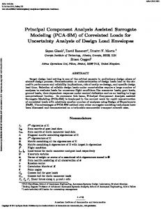
Fig. 1 Overview of surrogate contact model creation and implementation process. „a… 300 points „black dots… are sampled in the „X , ␪… design space. „b… Five static analyses using five axial loads are performed at each sample point location using an elastic foundation contact model to calculate Y and Fx. „c… Generalized Hertzian contact theory is used to model Fy as a function of Y while Fx is modeled as proportional to Fy. „d… The values of Y10 N, ky, ny, and ratio from the 300 sample points are fitted as functions of X and ␪ using Kriging. „e… During a dynamic simulation, the surrogate contact model calculates Fy and Fx from four Kriging models given the current values of X, Y, and ␪.

共2兲

from Eqs. 共2兲 and 共3兲 at any point during a dynamic simulation 共Fig. 1共e兲兲.

where Fˆy is the predicted SI contact force, ky is the contact stiffness, Y 10 N is the SI translation at contact initiation, and ny is the contact exponent. Use of Eq. 共2兲 to calculate Fˆy required fitting ky, Y 10 N, and ny as a function of X and ␪. Each of the 300 共X , ␪兲 sample pairs had five sampled values of Fy 共i.e., 10 N, 600 N, 1200 N, 1800 N, and 2400 N兲 and five associated output values of Y. Thus, Y 10 N was already known for each 共X , ␪兲 sample pair. To find ky and ny for each 共X , ␪兲 sample pair, we linearized Eq. 共2兲 by taking log10 of both sides and solved for log10共ky兲共and hence ky兲 and ny using linear least squares 共five equations in two unknowns兲. This process yielded one value of ky, Y 10 N, and ny for each 共X , ␪兲 sample pair. To calculate Fx, we used the observation that Fx is close to a constant fraction of Fy at each 共X , ␪兲 sample pair as follows:

Surrogate Contact Model Evaluation. To evaluate the computational speed and accuracy of our surrogate contact modeling approach, we performed nine dynamic wear simulations with both the surrogate contact model and the EF contact model used to generate it. Each wear simulation utilized different nominal component placements that were variations away from the original placements 共Fig. 2共a兲兲. The specific variations simulated were all possible combinations of three SI locations of the femoral flexion axis 共original⫾10 mm兲 and three AP slopes of the tibial insert 共original⫾10 deg兲. To cover all possible dynamic simulation paths, we specified the ranges of the 300 HQ sampling points using the limits of motion obtained from dynamic simulations performed with the EF contact model when the SI location of the femoral flexion axis and the AP slope of the tibial insert were set to their extreme values. We quantified differences between the sets of results by calculating root mean square errors 共RMSEs兲 in predicted contact forces, component translations, and wear volumes. Generation of wear volume predictions with the surrogate contact model required the development of a separate surrogate modeling approach based on prediction of medial and lateral center of pressure 共CoP兲 locations. This approach used Archard’s wear law 关45兴 to predict wear volume for any specified number of cycles from the time history of contact forces and CoP slip velocities on each side over a one-cycle dynamic simulation. Specifically,

Fˆy = ky共X, ␪兲关Y 10 N共X, ␪兲 − Y兴ny共X,␪兲

Fˆx = ratio共X, ␪兲Fˆy

共3兲

where Fˆx is the predicted AP contact force, “ratio” is the average of the five 共Fx , Fy兲 quotients obtained for each sample pair, and Fˆy is the SI contact force predicted by Eq. 共2兲. Thus, the final surrogate contact model utilized four separate Kriging models to fit ky, Y 10 N, ny, and ratio as a function of X and ␪ 共Fig. 1共d兲兲, permitting the calculation of Fˆy = f共X , Y , ␪兲 and Fˆx = f共X , ␪ , Fˆy兲 Journal of Biomechanical Engineering

APRIL 2009, Vol. 131 / 041010-3


Superior (+)/Inferior (-) Translation (m m)

a

b

10

A

B

C

D

E

F

Placement

0

Loads

-10

G

I

H

-10 0 10 Anterior(-)/Posterior(+) Slope (deg)

Motion

Fig. 2 Overview of global and local sensitivity analyses of predicted wear volume performed with the surrogate contact model. „a… Large variations in nominal component placements „labeled A–I… used for the global sensitivity analysis. „b… Small variations in component placements, input loads, and input motion used for local sensitivity analysis involving Monte Carlo methods applied to each nominal component placement.

n

V=N

2

兺兺 kF d

ij ij

i=1 j=1

n

= Nk

2

兺兺 F 兩v 兩⌬t ij

ij

共4兲

i=1 j=1

where V is the total wear volume of the medial and lateral sides over N cycles, N is the assumed total number of cycles 共5 ⫻ 106兲, i is a discrete time instant during the one-cycle dynamic simulation 共1 through n兲, j is the side 共medial or lateral兲, k is the assumed material wear rate 共1 ⫻ 10−7 mm3 / N m 关46兴兲, Fij is the contact force magnitude at time instant i on side j, and dij is the sliding distance of the CoP at time instant i on side j. Due to symmetry of the implant geometry, the predicted value of Fij on each side was taken as half the total contact force obtained from Eqs. 共2兲 and 共3兲. Prediction of dij on each side required determining the magnitude of the slip velocity vij of the CoP and multiplying by the time increment ⌬t 关4兴. To find vij, we used the kinematic concept of two points fixed on a rigid body 关47兴 vij = AvO + A␻B ⫻ pOCoP

共5兲

In this equation, A represents the tibial insert, B represents the femoral component, O is the femoral coordinate system origin located at the intersection of the flexion-extension and superiorinferior translation axes, CoP is the medial or lateral center of pressure location treated as a point fixed in body B, AvO is the velocity of point O with respect to reference frame A as determined from the relative translation of the femoral component origin, A␻␤ is the angular velocity of body B with respect to reference frame A as determined from the flexion-extension of the femoral component, and pOCoP is the position vector from point O to point CoP. While the values of AvO and A␻B were obtained directly from the dynamic simulations, calculation of the CoP location on each side required six additional Kriging models 共i.e., three components per side兲. Each Kriging model was created by fitting the average of the five CoP locations obtained from each 共X , ␪兲 sample pair. Wear volumes calculated by the surrogate contact model using the CoP-based approach were compared with those calculated by the EF contact model using both the CoPbased approach and a previously published element-based approach 关4,8兴 to verify that the surrogate model wear volume predictions were accurate. Surrogate Contact Model Application. As a practical application of the proposed surrogate contact modeling approach, we 041010-4 / Vol. 131, APRIL 2009

performed two types of sensitivity analyses to investigate how machine setup issues affect predicted wear volume. The first was a global sensitivity analysis to investigate the effect of large variations in component placements within the ranges defined in Fig. 2共a兲共i.e., ⫾10 mm/ deg兲. Specifically, we generated 400 combinations of component placements using 20 evenly spaced values of femoral flexion axis SI location and tibial insert AP slope. For each combination, the surrogate-based contact model was used to perform a dynamic simulation and predict wear volume. Percent changes in predicted wear volume were calculated relative to the maximum predicted value from all global sensitivity analysis results. The second category was a local sensitivity analysis to investigate the effect of small variations in nominal component placements and motion and load inputs by using Monte Carlo techniques 共Fig. 2共b兲兲. For the local sensitivity analysis, allowable variations in motion and load input curves were defined using experimental observations from eight different implant designs tested in a Stanmore simulator machine 关36兴. Deviations of the experimental input curves from the ISO standard curves were calculated and analyzed using principal component analysis 关48兴, with the first two principal components being sufficient to account for over 98% of the variability in each type of curve. These two components were used to generate new deviation curves by selecting component weights as uniformly distributed random numbers within the bounds of the experimental curves. These deviation curves were added to the ISO standard curves to create new input motion and load curves as needed for the Monte Carlo analyses. To distinguish between the effects of small errors in motion and load inputs and small errors in component placements, the local sensitivity analysis performed four types of Monte Carlo analyses for each of the nine nominal component placements for a total of 36 Monte Carlo analyses in all. Each type of Monte Carlo analysis varied input profiles and component placements separately or together. The first type varied motion and load profiles within 100% of their allowable ranges and also varied component placements within ⫾1 mm/ deg. The second type was similar but used smaller variations of only 10% of the allowable range for motion and load profiles and ⫾0.1 mm/ deg for component placements. The third type varied only motion and load profiles within 100% of their allowable ranges and imposed no variations on component placements. Finally, the fourth type varied component placements within ⫾1 mm/ deg but imposed no variations on motion and load Transactions of the ASME


0.2

0.2

RMSE (mm)

X

Y

0.15

0.15

0.1

0.1

0.05

0.05

0

0

4 RMSE (N)

Elastic foundation contact model

4 Fx

Fy

3

3

2

2

1

1

0

Table 1 Comparison between wear volume predictions „mm3… made with the elastic foundation contact model and the surrogate contact model for each of the nine nominal component placements. Each prediction was made for 5 Ã 106 motion cycles. Both contact models can predict wear volume using a simple center of pressure-based approach, while only the elastic foundation contact model can make predictions using a more detailed element-based approach.

A B C D E F G H I Nominal Placement

0

Nominal placement

Element-based

CoP-based

Surrogate contact model CoP-based

A B C D E F G H I

37.07 34.03 39.04 32.91 30.78 34.20 29.37 26.45 29.37

37.05 34.02 39.03 32.89 30.76 34.19 29.36 26.44 29.35

36.98 33.91 38.87 32.88 30.77 34.14 29.32 26.38 29.31

A B C D E F G H I Nominal Placement

Fig. 3 Root-mean-square errors in joint motions and contact forces for each nominal component placement. Errors are computed by comparing dynamic simulation results generated with the elastic foundation contact model and the surrogate contact model.

Results For the computational evaluation, the dynamic simulations performed with the surrogate contact model closely reproduced the planar motions, contact forces, and wear volumes predicted with the EF contact model for all nine component placements. On average, the RMSEs for planar motions and contact forces were less than 0.125 mm and 4 N, respectively 共Fig. 3兲. While each dynamic simulation performed with the EF contact model required approximately 13 min of CPU time, each simulation performed using the surrogate contact model required 13 s. For both the surrogate contact model and the EF contact model, the CoP-based approach for predicting wear volumes reproduced the elementbased EF results to within 0.5% error 共Table 1兲. For the practical application, the global and local sensitivity analyses revealed that large variations in component placements relative to the original locations and small variations in input motion relative to the ISO standard had a significant affect on predicted wear volume. For the global sensitivity analysis, predicted wear volume was sensitive to large variations in the SI location of the femoral flexion axis 共maximum change of 26% when the AP slope of tibial insert held fixed兲, the AP slope of the tibial insert 共maximum change of 13% when the SI location of femoral flexion axis held fixed兲, or both parameters simultaneously 共maximum change of 33%兲共Fig. 4兲. For the local sensitivity analysis, wear volume ranges were larger 共mean of 18 mm3 compared to 2 mm3兲 and 50% percentile wear volume results were lower 共mean of 23 mm3 compared to 31 mm3兲 when motion and load inputs and component placements were varied within 100% rather than 10% of their allowable ranges 共Figs. 5共a兲 and 5共b兲兲. When inputs and placements were varied separately within 100% of their allowable ranges, predicted wear volume was much more sensitive to motion and load inputs than to component placements 共maximum change of 64% compared to 5%; Figs. 5共c兲 and 5共d兲兲. Finally, when an additional global sensitivity analysis was performed with Journal of Biomechanical Engineering

Discussion Computational speed is a major limiting factor for performing sensitivity and optimization studies of total knee replacement designs. Unlike constraint-based joint models, knee joint contact models require repeated geometry evaluations that consume the vast majority of the CPU time in a dynamic contact simulation 关50兴. This paper has presented a novel surrogate modeling approach for performing efficient dynamic contact simulations of human joints. The surrogate contact model was developed to replace the original EF contact model to avoid time-consuming repeated evaluation of the surface geometry during dynamic simu-

Wear Volume (mm3)

profiles. For all types, percent changes in predicted wear volume were calculated relative to values obtained from the nominal component placements using the ISO standard inputs. Each Monte Carlo analysis was performed on a 3.4 GHz Pentium IV PC and involved at least 1000 dynamic contact simulations. The convergence criterion for each analysis was met when the mean and coefficient of variance 共i.e., 100 ⫻ standard deviation/mean兲 for the last 10% of the wear predictions were within 2% of the final mean and coefficient of variance 关49兴.

the original component placements to separate the influence of the different inputs, predicted wear volume varied approximately linearly with small changes in each input curve but was more sensitive to changes in flexion-extension motion 共maximum change of 47%; Fig. 6兲 than to changes in input loads 共maximum change of 20% for Fx and 14% for Fy; Figs. 6共a兲 and 6共b兲兲. Each Monte Carlo analysis performed with the surrogate contact model required 4 h of CPU time compared to an estimated 230 h with the EF contact model.

40

35

30 25 10

Sup

erio

10 g) r/Inf 0 0 e (de erio Slop r io r Tr r te ans -10 -10 /Pos (mm Anterior )

Fig. 4 Predicted wear volume as a function of large variations in component placements as calculated from 400 dynamic simulations performed with the surrogate contact model. Wear increases linearly when the femoral flexion axis is translated superiorly and quadratically when the tibial slope is increased anteriorly or posteriorly.

APRIL 2009, Vol. 131 / 041010-5


30

20

10

Wear Volume (mm3)

40

a

b

c

d

Wear Volume (mm3)

a

35

25

15 0

30

Fx 20

10

0

0.5

0.5

1

1

Flexion

b A B C D E F G H Nominal Placement

I

A B C D E F G H Nominal Placement

I

Fig. 5 Box plot distribution of predicted wear volume generated by four Monte Carlo analyses using the surrogate contact model. Each box has „from bottom to top… one whisker at the 10th percentile, three lines at the 25th, 50th, and 75th percentile, and another whisker at the 90th percentile. Outliers are indicated by black crosses located beyond the ends of the whiskers. For the first and second Monte Carlo analyses, motion and load inputs and component placements are varied together within „a… 100% or „b… 10% of their maximum ranges, respectively. For the third and fourth Monte Carlo analyses, „c… motion and load inputs or „d… component placements are varied separately within 100% of their maximum ranges, respectively.

lation. The surrogate contact model produced dynamic simulation and wear results that accurately matched those from the EF contact model but with an order of magnitude improvement in computational speed. This speed improvement would have been even more significant if a finite element contact model had been the original model. The 36 Monte Carlo analyses demonstrated how analyses that would have been impractical 共or at a minimum would have required extensive parallel processing兲 can be easily achieved on a single computer with the surrogate contact model. The sensitivity results also have practical value, suggesting that wear volume generated by simulator machines may be sensitive to large variations in component placements within the machine as well as small variations in the flexion-extension motion input to the machine. The primary benefit of using surrogate contact models in dynamic simulations is improved computational efficiency. For elastic foundation or finite element contact models, the computation time per dynamic simulation is largely determined by the number of deformable contacts in the model. Thus, a musculoskeletal computer model utilizing deformable contact models for multiple joints could easily require hours or days of CPU time to complete a single dynamic simulation. Repeated dynamic simulations as part of a sensitivity or optimization study would become impractical. By using surrogate contact models instead, one could eliminate the computational cost of the contact solver as the limiting factor. The larger the number of deformable contacts in a multibody dynamic model, the greater the anticipated benefit from using surrogate contact models. While we have shown that surrogate contact models can be beneficial for sensitivity studies, the greatest computational benefit is likely to occur for optimization studies. For stochastic sensitivity studies, statistically based alternatives to Monte Carlo analyses exist that require fewer repeated simulations. For example, Laz et al. 关51兴 used the mean value method 关52兴 to perform probabilistic elastic foundation simulations of a TKR design and reduced the number of simulations by a factor of 4 compared to a 041010-6 / Vol. 131, APRIL 2009

Wear Volume (mm3)

Wear Volume (mm3)

40

35

25

15 0 0 0.5

Fy

0.5 1 1

Flexion

Fig. 6 Predicted wear volume as a function of variations in „a… anterior-posterior load and femoral flexion angle and „b… axial load and femoral flexion angle. Both plots were created by performing dynamic simulations with the surrogate model and changing the weight of the first principal component for each input profile variation away from the ISO standard. Each weight was normalized to be between 0 and 1. The cross marker „ⴛ… represents the ISO standard input with no superimposed input profile variations „i.e., weights of 0… while the circle marker „䊊… represents the ISO standard input with maximum superimposed input profile variations „i.e., weights of 1….

traditional Monte Carlo approach. Since the CPU time per simulation was 6 min, the use of a surrogate contact model could still reduce the overall computation time by an additional factor of 28, assuming we could achieve comparable speed improvements for the 3D situation. In contrast, no good methods exist for reducing the number of simulations in optimization studies. For those situations, the factor of 60 reduction in computation time 共i.e., 13 min– 13 s兲 could mean the difference between an impossible and an achievable optimization study. Other than computational efficiency, surrogate contact models possess the additional benefits of being adaptable and flexible. First, the surrogate-based contact modeling approach presented here is not limited to the knee joint. Theoretically, the approach could be applied to any joint contact model whose input-output relationships can be sampled. The modified HQ sampling method should be suitable for any joint contact model once the sensitive directions are identified. Therefore, neither type of joint 共e.g., hip or knee or ankle兲 nor type of contact model 共e.g., EF or finite element兲 nor type of material model 共e.g., linear or nonlinear兲 is critical for developing a surrogate contact model. The benefit of using an EF contact model to generate the required sample points was that it is relatively fast computationally for performing repeated static analyses. Finite element models would require more time for each static analysis, plus the inputs are usually applied displacements rather than loads. For the finite element situation, it could be necessary to curve fit the force-displacement curve at each sample point to produce new points at fixed force increTransactions of the ASME


ments. Second, the surrogate contact model represents the real surface geometry implicitly within the design space. Since the surrogate modeling approach uses the real surface geometry to generate the sampling points, no idealization of complex surface geometry is required. Third, the approach is not limited to a single surrogate model fitting method. While we used Kriging in the present study, any of the fitting methods mentioned previously could be investigated as well 关24,26,53,54兴. Though polynominal response surfaces are the most commonly used surrogate model, Kriging has the advantage of interpolating the sample point outputs, which is appealing for deterministic computer models 关15,54兴. The global sensitivity results demonstrate the importance of developing a standardized method for defining the location of the femoral flexion axis. For a given tibial slope, predicted wear volume varied approximately linearly with changes in the superiorinferior location of the femoral flexion axis, increasing as the axis was translated superiorly 共Fig. 4兲. Superior translation of the flexion axis increases the distance to the CoP, thereby increasing the magnitude of the slip velocity in Eq. 共4兲. Thus, to minimize wear for any given implant design, one can simply locate the femoral flexion axis close to the articular surfaces. In contrast, the predicted wear volume varied approximately quadratically with changes in tibial slope, increasing as the insert was tilted anteriorly or posteriorly away from its neutral position 共Fig. 4兲. Increasing the tibial anterior or posterior slope increases the AP tibial sliding distance 关55兴, thereby leading to an increase in predicted wear volume 关56,57兴. In contrast, the local sensitivity results demonstrate the importance of controlling machine inputs closely, especially the femoral flexion angle. The Monte Carlo analyses and the additional global sensitivity analysis revealed when small variations were imposed on the input motion, loads, and component placements, only variations in the femoral flexion angle resulted in large changes in predicted wear volume. When the flexion angle was varied within 100% of its allowable range, the drop in 50th percentile wear volume results 共Figs. 5共a兲 and 5共c兲兲 relative to the ISO standard inputs 共i.e., 50% percentile results in Figs. 5共b兲 and 5共d兲兲 was due to the use of imposed variations that always reduced the amplitude of the curve 关36兴. This finding is consistent with previous studies showing that predicted wear volume decreases when the amplitude of the input curves is reduced 关58–60兴. Thus, another way to minimize wear for any given implant design is to use a control system that systematically undershoots the peaks in the input flexion-extension curve. Combining this approach with an inferiorly located femoral flexion axis could cut wear volume by more than 50% compared to the original component placement with ISO standard inputs. The development of a standard for acceptable variations in input flexion-extension motion should be considered as well. Despite its computational advantages, the proposed surrogate contact modeling approach possesses several important limitations. The biggest one is that new surrogate contact models must be generated if implant geometry, insert thickness, or material properties are changed, at least for the current formulation. The geometry limitation makes it impossible to use surrogate contact models for progressive wear simulations, where the surface geometry is changed gradually over an iterative sequence of wear simulations. However, this limitation is not serious if only wear volume is of interest, as recent progressive wear simulation studies have reported that predicted wear volume 共but not wear area or depth兲 is relatively insensitive to whether or not the surface geometry is changed gradually 关8,9兴. Theoretically, changes in insert thickness or material model parameter values could be accommodated by adding more input variables to the surrogate model fitting process 共e.g., make insert thickness an additional surrogate model input兲. For contact forces, a changing value of Young’s modulus 共E兲 in a linear elastic material model can be accommodated without adding another input variable. If all sample points Journal of Biomechanical Engineering

are generated using a value of E = 1, then the contact force output by the surrogate model can be scaled by the desired value of E 关29兴. A number of other limitations exist as well. First, the current surrogate contact model is restricted to sagittal plane motion, where contact force is dominated by SI translation of the femoral component. For 3D simulations, contact force will be highly sensitive to changes in varus-valgus rotation as well 关40兴. In addition to an increased number of sensitive directions, the number of sample points will also need to increase. However, the increased computational cost for evaluating more sample points is paid up front since the sampling process is only performed once. Second, the calculation of Fx is dependent on the value of Fy computed from Eq. 共2兲. Thus, the quality of the Fy prediction will directly impact the Fx calculation. The current approach works fine for sagittal plane models with a single sensitive direction, but an independent calculation of Fx may be needed for 3D situations where more than one sensitive direction is present. Third, the CoP approach for calculating wear volume may not work well for some types of 3D motion. For example, for a sphere spinning about a vertical axis while in contact with a plane, the CoP would be located at the bottom of the sphere where the slip velocity is zero. Thus, no wear volume would be calculated, even though the element-based approach would calculate a nonzero wear volume based on the pressures and slip velocities throughout the contact area. Consequently, the CoP approach will work well for analysis of TKR designs undergoing 3D motion only if the amount of internal-external rotation is “small.” Fourth, our Monte Carlo results are limited to cruciate-retaining designs with a nonconformal tibial insert. Whether or not our conclusions are generalizable to other implant designs and simulator machines would require further investigation. In summary, this paper has demonstrated that surrogate contact modeling can significantly improve the computational speed of dynamic contact simulations and is appropriate for 2D sensitivity and optimization studies incorporating deformable contact. Refinement of the current 2D approach and extension to 3D problems are topics of ongoing research. Once surrogate contact models are developed for 3D situations, it should be possible to create dynamic musculoskeletal models with multiple deformable joints that can be simulated in a short amount of CPU time. Such models should improve our ability to analyze new knee implant designs rapidly and to predict muscle forces across joints where contact forces may have an important stabilizing effect.

Acknowledgment This work was supported by an NSF CBET grant to B.J.F. and R.T.H.

Appendix Below we provide links to the MATLAB software tools used in this study to develop surrogate contact models. Hammersley Quasirandom Sampling: http://people.scs.fsu.edu/~burkardt/m_src/hammersley/ hammersley.html DACE Kriging Toolbox: http://www2.imm.dtu.dk/~hbn/dace/

References 关1兴 Noble, P. C., Gordon, M. J., Weiss, J. M., Reddix, R. N., Conditt, M. A., and Mathis, K. B., 2005, “Does Total Knee Replacement Restore Normal Knee Function?,” Clin. Orthop. Relat. Res., 431, pp. 157–165. 关2兴 Mancuso, C. A., Sculco, T. P., Wickiewicz, T. L., Jones, E. C., Robbins, L., Warren, R. F., and Williams-Russo, P., 2001, “Patients’ Expectations of Knee Surgery,” J. Bone Jt. Surg., Am. Vol., 83A共7兲, pp. 1005–1012. 关3兴 Weiss, J. M., Noble, P. C., Conditt, M. A., Kohl, H. W., Roberts, S., Cook, K. F., Gordon, M. J., and Mathis, K. B., 2002, “What Functional Activities Are Important to Patients With Knee Replacements?,” Clin. Orthop. Relat. Res., 40共4兲, pp. 172–188. 关4兴 Fregly, B. J., Sawyer, W. G., Harman, M. K., and Banks, S. A., 2005, “Com-

APRIL 2009, Vol. 131 / 041010-7


关5兴关6兴关7兴关8兴

关9兴

关10兴

关11兴关12兴关13兴

关14兴关15兴关16兴关17兴关18兴

关19兴关20兴关21兴


关26兴关27兴


putational Wear Prediction of a Total Knee Replacement From In Vivo Kinematics,” J. Biomech., 38共2兲, pp. 305–314. Giddings, V. L., Kurtz, S. M., and Edidin, A. A., 2001, “Total Knee Replacement Polyethylene Stresses During Loading in a Knee Simulator,” ASME J. Tribol., 123共4兲, pp. 842–847. Halloran, J. P., Petrella, A. J., and Rullkoetter, P. J., 2005, “Explicit Finite Element Modeling of Total Knee Replacement Mechanics,” J. Biomech., 38共2兲, pp. 323–331. Rawlinson, J. J., Furman, B. D., Li, S., Wright, T. M., and Bartel, D. L., 2006, “Retrieval, Experimental, and Computational Assessment of the Performance of Total Knee Replacements,” J. Orthop. Res., 24共7兲, pp. 1384–1394. Zhao, D., Sakoda, H., Sawyer, W. G., Banks, S. A., and Fregly, B. J., 2008, “Predicting Knee Replacement Damage in a Simulator Machine Using a Computational Model With a Consistent Wear Factor,” ASME J. Biomech. Eng., 130共1兲, p. 011004. Knight, L. A., Pal, S., Coleman, J. C., Bronson, F., Haider, H., Levine, D. L., Taylor, M., and Rullkoetter, P. J., 2007, “Comparison of Long-Term Numerical and Experimental Total Knee Replacement Wear During Simulated Gait Loading,” J. Biomech., 40共7兲, pp. 1550–1558. Halloran, J. P., Easley, S. K., Petrella, A. J., and Rullkoetter, P. J., 2005, “Comparison of Deformable and Elastic Foundation Finite Element Simulations for Predicting Knee Replacement Mechanics,” ASME J. Biomech. Eng., 127共5兲, pp. 813–818. Box, G. E. P., and Draper, N. R., 1987, “Empirical Model-Building and Response Surfaces,” Applied Probability and Statistics 共Wiley Series in Probability and Mathematical Statistics兲, Wiley, New York. Khuri, A. I., and Cornell, J. A., 1996, Response Surfaces: Designs and Analyses, Statistics, Textbooks and Monographs, Dekker, New York. Myers, R. H., and Montgomery, D. C., 1995, “Response Surface Methodology: Process and Product in Optimization Using Designed Experiments,” Applied Probability and Statistics 共Wiley Series in Probability and Statistics兲, Wiley, New York. Jones, D. R., Schonlau, M., and Welch, W. J., 1998, “Efficient Global Optimization of Expensive Black-Box Functions,” J. Global Optim., 13共4兲, pp. 455– 492. Sacks, J., Welch, W. J., Mitchell, T. J., and Wynn, H. P., 1989, “Design and Analysis of Computer Experiments,” Stat. Sci., 4共4兲, pp. 409–435. Chen, S., Chng, E. S., and Alkadhimi, K., 1996, “Regularized Orthogonal Least Squares Algorithm for Constructing Radial Basis Function Networks,” Int. J. Control, 64共5兲, pp. 829–837. Wendland, H., 1995, “Piecewise Polynomial, Positive Definite and Compactly Supported Radial Basis Functions of Minimal Degree,” Adv. Comput. Math., 4共1兲, pp. 389–396. Wahba, G., 1987, “Spline Models for Observational Data,” CBMS-NSF Regional Conference Series in Applied Mathematics, Based on a Series of Ten Lectures at Ohio State University at Columbus, Mar. 23–27, Society for Industrial and Applied Mathematics, Philadelphia, PA. Girosi, F., 1998, “An Equivalence Between Sparse Approximation and Support Vector Machines,” Neural Comput., 10共6兲, pp. 1455–1480. Vapnik, V. N., Statistical Learning Theory, Wiley, New York. Cox, S. E., Haftka, R. T., Baker, C. A., Grossman, B., Mason, W. H., and Watson, L. T., 2001, “A Comparison of Global Optimization Methods for the Design of a High-Speed Civil Transport,” J. Global Optim., 21共4兲, pp. 415– 433. Koch, P. N., Simpson, T. W., Allen, J. K., and Mistree, F., 1999, “Statistical Approximations for Multidisciplinary Design Optimization: The Problem of Size,” J. Aircr., 36共1兲, pp. 275–286. Liu, B., Haftka, R. T., and Akgun, M. A., 2000, “Two-Level Composite Wing Structural Optimization Using Response Surfaces,” Struct. Multidiscip. Optim., 20共2兲, pp. 87–96. Queipo, N. V., Haftka, R. T., Shyy, W., Goel, T., Vaidyanathan, R., and Tucker, P. K., 2005, “Surrogate-Based Analysis and Optimization,” Prog. Aerosp. Sci., 41共1兲, pp. 1–28. Queipo, N. V., Pintos, S., Rincon, N., Contreras, N., and Colmenares, J., 2002, “Surrogate Modeling-Based Optimization for the Integration of Static and Dynamic Data Into a Reservoir Description,” J. Pet. Sci. Eng., 35共3–4兲, pp. 167–181. Wang, G. G., and Shan, S., 2007, “Review of Metamodeling Techniques in Support of Engineering Design Optimization,” ASME J. Mech. Des., 129共4兲, pp. 370–380. Bouzid, A. H., De Technologie Superieure, E., and Champliaud, H., 1998, “On the Use of Dual Kriging Interpolation for the Evaluation of the Gasket Stress Distribution in Bolted Joints,” Proceedings of the ASME Pressure Vessels and Piping Conference, Vol. 457, pp. 77–83. Chang, P. B., Williams, B. J., Santner, T. J., Notz, W. I., and Bartel, D. L., 1999, “Robust Optimization of Total Joint Replacements Incorporating Environmental Variables,” ASME J. Biomech. Eng., 121共3兲, pp. 304–310. Lin, Y. C., Farr, J., Carter, K., and Fregly, B. J., 2006, “Response Surface Optimization for Joint Contact Model Evaluation,” J. Appl. Biomech., 22共2兲, pp. 120–130. An, K. N., Himenso, S., Tsumura, H., Kawai, T., and Chao, E. Y. S., 1990, “Pressure Distribution on Articular Surfaces: Application to Joint Stability Analysis,” J. Biomech., 23共10兲, pp. 1013–1020. Blankevoort, L., Kuiper, J. H., Huiskes, R., and Grootenboer, H. J., 1991, “Articular Contact in a Three-Dimensional Model of the Knee,” J. Biomech.,

041010-8 / Vol. 131, APRIL 2009

24共11兲, pp. 1019–1031. 关32兴 Fregly, B. J., Bei, Y. H., and Sylvester, M. E., 2003, “Experimental Evaluation of an Elastic Foundation Model to Predict Contact Pressures in Knee Replacements,” J. Biomech., 36共11兲, pp. 1659–1668. 关33兴 Li, G. A., Sakamoto, M., and Chao, E. Y. S., 1997, “A Comparison of Different Methods in Predicting Static Pressure Distribution in Articulating Joints,” J. Biomech., 30共6兲, pp. 635–638. 关34兴 Pandy, M. G., Sasaki, K., and Kim, S., 1998, “A Three-Dimensional Musculoskeletal Model of the Human Knee Joint. Part 1: Theoretical Construct,” Comput. Methods Biomech. Biomed. Eng., 1共2兲, pp. 87–108. 关35兴 Walker, P. S., Blunn, G. W., Broome, D. R., Perry, J., Watkins, A., Sathasivam, S., Dewar, M. E., and Paul, J. P., 1997, “A Knee Simulating Machine for Performance Evaluation of Total Knee Replacements,” J. Biomech., 30共1兲, pp. 83–89. 关36兴 Desjardins, J. D., Walker, P. S., Haider, H., and Perry, J., 2000, “The Use of a Force-Controlled Dynamic Knee Simulator to Quantify the Mechanical Performance of Total Knee Replacement Designs During Functional Activity,” J. Biomech., 33共10兲, pp. 1231–1242. 关37兴 Hammersley, J. M., 1960, “Related Problems .3. Monte-Carlo Methods for Solving Multivariable Problems,” Ann. N.Y. Acad. Sci., 86共3兲, pp. 844–874. 关38兴 Diwekar, U. M., 2003, Introduction to Applied Optimization, Springer, New York. 关39兴 Kalagnanam, J. R., and Diwekar, U. M., 1997, “An Efficient Sampling Technique for Off-Line Quality Control,” Technometrics, 39共3兲, pp. 308–319. 关40兴 Fregly, B. J., Banks, S. A., D’lima, D. D., and Colwell, C. W., Jr., 2008, “Sensitivity of Knee Replacement Contact Calculations to Kinematic Measurement Errors,” J. Orthop. Res., 26共9兲, pp. 1173–1179. 关41兴 Cressie, N., 1992, “Statistics for Spatial Data,” Terra Nova, 4共5兲, pp. 613–617. 关42兴 Gupta, A., Ding, Y., Xu, L., and Reinikainen, T., 2006, “Optimal Parameter Selection for Electronic Packaging Using Sequential Computer Simulations,” ASME J. Manuf. Sci. Eng., 128共3兲, pp. 705–715. 关43兴 Lophaven, S. N., Nielsen, H. B., and Søndergaard, J., 2002, “Dace—A Matlab Kriging Toolbox,” Technical Report No. IMM-TR-2002-13, Informatics and Mathematical Modelling, Technical University of Denmark. 关44兴 Johnson, K. L., 1987, Contact Mechanics, Cambridge University Press, Cambridge. 关45兴 Archard, J. F., and Hirst, W., 1956, “The Wear of Metals Under Unlubricated Conditions,” Proc. R. Soc. London, Ser. A, 236共1206兲, pp. 397–410. 关46兴 Fisher, J., Dowson, D., Hamdzah, H., and Lee, H. L., 1994, “The Effect of Sliding Velocity on the Friction and Wear of Uhmwpe for Use in Total Artificial Joints,” Wear, 175共1–2兲, pp. 219–225. 关47兴 Kane, T. R., and Levinson, D. A., 1985, Dynamics, Theory and Applications 共Series in Mechanical Engineering兲, McGraw-Hill, New York. 关48兴 Daffertshofer, A., Lamoth, C. J. C., Meijer, O. G., and Beek, P. J., 2004, “PCA in Studying Coordination and Variability: A Tutorial,” Clin. Biomech., 19共4兲, pp. 415–428. 关49兴 Valero-Cuevas, F. J., Johanson, M. E., and Towles, J. D., 2003, “Towards a Realistic Biomechanical Model of the Thumb: The Choice of Kinematic Description May Be More Critical Than the Solution Method or the Variability/ Uncertainty of Musculoskeletal Parameters,” J. Biomech., 36共7兲, pp. 1019– 1030. 关50兴 Bei, Y. H., and Fregly, B. J., 2004, “Multibody Dynamic Simulation of Knee Contact Mechanics,” Med. Eng. Phys., 26共9兲, pp. 777–789. 关51兴 Laz, P. J., Pal, S., Halloran, J. P., Petrella, A. J., and Rullkoetter, P. J., 2006, “Probabilistic Finite Element Prediction of Knee Wear Simulator Mechanics,” J. Biomech., 39共12兲, pp. 2303–2310. 关52兴 Wu, Y. T., Millwater, H. R., and Cruse, T. A., 1990, “Advanced Probabilistic Structural-Analysis Method for Implicit Performance Functions,” AIAA J., 28共9兲, pp. 1663–1669. 关53兴 Jin, R., Chen, W., and Simpson, T. W., 2001, “Comparative Studies of Metamodelling Techniques Under Multiple Modelling Criteria,” Struct. Multidiscip. Optim., 23共1兲, pp. 1–13. 关54兴 Simpson, T. W., Peplinski, J. D., Koch, P. N., and Allen, J. K., 2001, “Metamodels for Computer-Based Engineering Design: Survey and Recommendations,” Eng. Comput., 17共2兲, pp. 129–150. 关55兴 Bai, B., Baez, J., Testa, N. N., and Kummer, F. J., 2000, “Effect of Posterior Cut Angle on Tibial Component Loading,” J. Arthroplasty, 15共7兲, pp. 916– 920. 关56兴 Blunn, G. W., Walker, P. S., Joshi, A., and Hardinge, K., 1991, “The Dominance of Cyclic Sliding in Producing Wear in Total Knee Replacements,” Clin. Orthop. Relat. Res., 273, pp. 253–260. 关57兴 Kawanabe, K., Clarke, I. C., Tamura, J., Akagi, M., Good, V. D., Williams, P. A., and Yamamoto, K., 2001, “Effects of a-P Translation and Rotation on the Wear of Uhmwpe in a Total Knee Joint Simulator,” J. Biomed. Mater. Res., 54共3兲, pp. 400–406. 关58兴 Barnett, P. I., Fisher, J., Auger, D. D., Stone, M. H., and Ingham, E., 2001, “Comparison of Wear in a Total Knee Replacement Under Different Kinematic Conditions,” J. Mater. Sci.: Mater. Med., 12共10–12兲, 1039–1042. 关59兴 D’lima, D. D., Hermida, J. C., Chen, P. C., and Colwell, C. W., 2001, “Polyethylene Wear and Variations in Knee Kinematics,” Clin. Orthop. Relat. Res., 392, pp. 124–130. 关60兴 Johnson, T. S., Laurent, M. P., Yao, J. Q., and Gilbertson, L. N., 2001, “The Effect of Displacement Control Input Parameters on Tibiofemoral Prosthetic Knee Wear,” Wear, 250, pp. 222–226.

Transactions of the ASME
