performance measure to asses the accuracy of the surrogate model.2 .... aThe SUMO Toolbox can be downloaded from: http://sumo.intec.ugent.be. ..... search strategy is relatively dimension-free, more work is needed to investigate the impact ...
Inverse surrogate modeling: output performance space sampling Ivo Couckuyt∗ and Dirk Gorissen∗
Tom Dhaene† and Filip De Turck†
Ghent University-IBBT, Ghent, 9050, Belgium
Ghent University-IBBT Ghent, 9050, Belgium
The use of Surrogate Based Optimization (SBO) is widely spread in engineering design to find optimal performance characteristics of computational expensive simulation codes (i.e., the forward problem). However, often the practitioner knows a priori the desired performance and is interested in finding the associated design parameters (i.e., the inverse problem). A popular method to solve such reverse (inverse) problems is to minimize the error between the simulated performance and the desired goal performance. While this works quite well, it only allows for the identification of one design, namely, the global optimum according to the error function. In this paper, the authors propose a method to sample a whole range of performances using surrogate models. This technique, based on the probability of improvement criterion and kriging models, is successfully demonstrated on the branin function to obtain a quasi-uniform set of samples that lie in a predefined output range.
I.
Introduction
This paper is concerned with efficiently solving complex, computational expensive problems using surrogate modeling techniques.1 Surrogate models, also known as metamodels, are cheap approximation models for computational expensive (black-box) simulations. Surrogate modeling techniques are wellsuited to handle, for example, expensive finite element (FE) simulations, computational fluid dynamic (CFD) simulations and, of course, physical experiments. Depending on the construction and usage of surrogate models several modeling flavors can be distinguished. Surrogate models can be built upfront to approximate the simulation code accurately over the entire input space and, hence, can afterwards be used to replace the expensive code for design, analysis and optimization purposes. On the other hand, the construction of surrogate models can also be integrated in the optimization process. Usually, the latter case, known as Surrogate Based Optimization (SBO), generates surrogate models on the fly that are only accurate in certain regions of the input space, e.g., around optimal regions. The construction of surrogate models as efficiently as possible is an entire research domain in itself. In order to come to an acceptable model, numerous problems and design choices need to be overcome (what data collection strategy to use, which variables are relevant, how to integrate domain knowledge, etc.). Other aspects of surrogate modeling include choosing the right type of approximation model for the problem at hand, a tuning strategy for the surrogate model parameters (=hyperparameters), and a performance measure to asses the accuracy of the surrogate model.2 The general work-flow of surrogate modeling is illustrated in Figure 1. First, an experimental design, e.g., from Design of Experiments (DOE), is specified and evaluated. Subsequently, surrogate models are built to fit this data as good as possible, according to a set of measures (e.g., cross validation). The hyperparameters are estimated using an optimization algorithm. The accuracy of the set of surrogate models is improved until no further improvement can be obtained (or when another stopping criterion, such as a time limit, is met). If the stopping criteria are satisfied the process is halted and the final, best surrogate model is returned. On the other hand, when no stopping criterion is met, a sequential design strategy, also known as active learning or adaptive sampling, will select new samples to be evaluated and the surrogate models are updated with this new data. Most often, surrogate models are used to solve so-called forward problems. The practitioner is interested in the output or performance characteristics of the simulation system given the input parameters. ∗ PhD student, Department of Information Technology (INTEC), Ghent University-IBBT, Gaston Crommenlaan 8, Ghent, 9050, Belgium, AIAA student member. † Professor, Department of Information Technology (INTEC), Ghent University-IBBT, Gaston Crommenlaan 8, Ghent, 9050, Belgium.
1 of 9 American Institute of Aeronautics and Astronautics
Figure 1: Flow chart of the surrogate modeling process.
The surrogate models define the mapping between the input space (design space) and the output space (performance space). In contrast, the focus of the reverse (inverse) problem is on exploring the input space. Ideally, a surrogate model could be created that maps the output parameters to the input parameters (as opposite to forward modeling) of the complex system over the entire input space. However, many inverse problems are typically ill-posed. Considering Hadamard’s definition of ill-posedness,3 the two outstanding problems hampering the creation of a full inverse surrogate model are non-uniqueness and instability. A good overview of the associated intricacies is presented by Barton in.4 For all the above reasons, the inverse problem is often reduced to the task of finding one (or more) input parameter combination for a certain output characteristic. Still, it is possible that, 1. no such input parameter combination exists 2. more than one input parameter combination satisfies the given output characteristic. A typical inverse problem is the estimation of some (physical) material or design parameter, e.g., the permittivity of a substrate5 or the elasticity of rubber,6 given the desired output or system behavior. A popular solution is to convert the reverse problem to a (forward) optimization problem. Namely, a simulation model is constructed, parametrized by the properties or design parameters of interest. By minimizing the error between the parametrized simulation model and the measured data the input parameters (material properties) of the simulation model are obtained that correspond with the measurements or desired output, see Figure 2.
Figure 2: The inverse problem is often solved by minimizing the error function between the simulation output and the measured data. The focus of this paper is to efficiently solve inverse problems directly, i.e., identifying the regions in the input space that correspond to the desired output value(s). The contribution of this paper is a novel method, i.e., a sequential design step in surrogate modeling, that is able to efficiently sample the (disconnected) input regions, in a quasi-uniform way. The surrogate model of choice is the Gaussian Process (GP) based kriging. Kriging is a popular surrogate model for the approximation of deterministic
2 of 9 American Institute of Aeronautics and Astronautics
computer code.7 GP enable the use of statistical infill criteria in the sequential design strategy. The presented method consists of the extension of such a statistical infill criterion, namely, the Probability of Improvement (PoI),8 and a new search strategy to exploit the infill criterion. This approach has been implemented in a flexible research platform for surrogate modeling, the SUrrogate MOdeling (SUMO) Toolboxa ,2 and is illustrated on the branin function. Section II describes the use of infill criteria and in particular the generalization of the PoI criterion. A new search strategy to exploit infill criteria is described in section III. This approach is demonstrated on the branin function. Details of the setup are found in section IV. Results and conclusion form the last two sections of this paper, i.e., sections V and VI.
II.
Infill criteria
In engineering, infill criteria are (sampling) functions, also known as figures of merit or metrics, that measure how interesting a data point is in the input space. Starting from an initial approximation of the simulation system, new sample points (infill or update points) are selected based on an infill criterion. The variety of infill criteria ranges from the accuracy of the prediction (e.g., for creating globally accurate surrogate models) to the prediction itself (e.g., to facilitate optimization). In global SBO it is crucial that the infill criterion is a balance between explorationb and exploitationc . A well-known infill criterion that is able to effectively solve this exploitation/exploration trade-off is Expected Improvement (EI), which has been popularized by Jones et al.9, 10 as the Efficient Global Optimization (EGO) algorithm. Jones wrote an excellent discussion regarding the infill criteria approach in.8 Subsequently, Sasena compared different infill criteria for optimization and investigated extensions of those infill criteria for constrained optimization problems in.11 A.
Probability of Improvement (PoI)
Among several statistical infill criteria investigated by Jones the PoI is the focus of this work. The PoI equation (1), defined below, can be interpreted graphically (see Figure 3). At x = 0.5, a Gaussian probability density function is drawn and expresses the uncertainty about the predicted function value of a sampled and unknown function y = f (x). Thus, the uncertainty at any point x is treated as the realization of a random variable Y (x) with mean yˆ = fˆ(x) (= prediction) and variance sˆ2 = σ ˆ 2 (x) (= prediction variance). Assuming the random variable Y (x) is normally distributed, then the shaded area under the Gaussian probability density function is the P oI of any newly calculated function value f (x) over the intermediate minimum function value fmin (the dotted line). PoI is denoted as P (Y (x) ≤ fmin ), i.e., fZmin
P oI = P (Y (x) ≤ fmin ) =
Y (x) dY −∞
� =Φ
� fmin − yˆ , sˆ
(1)
h � �i where Φ(t) is the standard normal cumulative distribution function Φ(t) = 12 1 + erf √t2 and erf (·) is the error function. PoI or any other statistical infill criteria (e.g., EI) are optimized over x to find the subsequent data point to evaluate. Note, however, that besides the prediction yˆ = fˆ(x) of the surrogate model, a pointwise variance estimation sˆ2 = σ ˆ 2 (x) of the surrogate is also required. Both predictions (ˆ y and sˆ2 ) are provided by the kriging surrogate model. B.
Generalized Probability of Improvement (gPoI)
While PoI is a very useful infill criterion for optimization, it only focuses on the global optimum, not on a range of output values. The authors extend the idea of the PoI criterion to allow identification of an arbitrarily band in the output space. Let [T1 , T2 ] be the range of interest in the output space. Then the probability that the function value f (x) of a point x lies in this range is defined as: a The SUMO Toolbox can be downloaded from: http://sumo.intec.ugent.be. An AGPL open source license is available for research purposes. b exploration = enhancing the overall accuracy of the surrogate model c exploitation = enhancing the accuracy of the surrogate model solely in the region of the (current) optimum
3 of 9 American Institute of Aeronautics and Astronautics
1.5 Unknown model Data points f(xi) 1
f(x)
0.5
Minimum over all data points: fmin Surrogate model Gaussian PDF at x=0.5 Prediction mean at x=0.5 PoI at x=0.5
0 fmin −0.5
−1
−1.5 −1
−0.5
0
0.5
1
1.5
x
Figure 3: Graphical illustration of a Gaussian Process and Probability of Improvement (PoI). A surrogate model (dashed line) is constructed based on some data points (circles). For each point the surrogate model predicts a Gaussian probability density function (PDF). E.g., at x = 0.5 an example of such a PDF is drawn. The volume of the shaded area is the PoI over the minimum function value fmin .
ZT2 gP oI(x) = P (T1 ≤ Y (x) ≤ T2 ) =
Y (x) dY T1
= P (T2 ≤ Y (x)) − P (T1 ≤ Y (x)) ZT2
ZT1 Y (x) dY −
= −∞
Y (x) dY −∞
� T1 − yˆ , (2) sˆ h � �i where Φ(t) is the standard normal cumulative distribution function Φ(t) = 12 1 + erf √t2 and erf (·) is the error function. This criterion represents the probability that a new point x is in the desired output interval [T1 , T2 ]. Hence, the abbreviation “PoI” is not completely correct anymore as the focus is now on sampling an interval instead of improving the optimum. Unlike PoI, the gPoI cannot be simply optimized to identify new samples. Existing samples that are already lying in the output range [T1 , T2 ] have probability one (see Figure 6a), and, hence, straightforward optimization of the criterion will result in duplicate samples. Other (space-filling) strategies have to be devised that makes fully use of the information provided by gPoI. In fact, note that this is actually a constrained sampling problem . If uncertainty was not taken into account a simple constraint would suffice, i.e., c(x) = T1 ≤ f (x) ≤ T2 . By taking uncertainty in account, (new) regions of interest may be identified faster and more accurately. �
=Φ
III.
T2 − yˆ sˆ
�
�
−Φ
Search strategies
The techniques explained in the previous sections are all utility functions. Such utility functions are used to identify interesting new points in a sequential design strategy. Various search strategies exist to exploit the utility functions. For instance, the original EGO algorithm9 simply optimizes the EI. In particular, the deterministic branch and bound methodology was used to find the global optimum. To that end, a convex upper bound had to be calculated for the EI. However, if one wants to use other utility functions (or other types of
4 of 9 American Institute of Aeronautics and Astronautics
1.5 Unknown model Data points f(xi) 1
f(x)
0.5
Desired output range [T1 T2] Surrogate model Gaussian PDF at x=0.5 Prediction mean at x=0.5 P(I(x=0.5)) T2
0 T1
−0.5
−1
−1
−0.5
0
0.5
1
1.5
x
Figure 4: Graphical illustration of a Gaussian Process and the generalized Probability of Improvement (gPoI). A surrogate model (dashed line) is constructed based on some data points (circles). For each point the surrogate model predicts a Gaussian probability density function (PDF). E.g., at x = 0.5 an example of such a PDF is drawn. The volume of the shaded area is the gPoI based on the desired output range [T1 , T2 ].
surrogate models) this upper bound must be redefined. In later work more black-box optimization methods were used with similar results, e.g., the DIviding REctangles (DIRECT)12 or an extensive pattern search. Moreover, multi-modal optimization methods are suggested in literature (e.g., in13, 14 ) to select multiple samples in one iteration, taking full advantage of parallel computing. Global optimization methods are not suited to directly exploit the new gPoI criterion because there might exist multiple (or even an infinite number of) solutions. Therefore the authors adapt a generic sampling framework for sequential design. The algorithmic flow is depicted in Figure 5. The search strategy is configured as followed: First, n candidate samples are drawn from the uniform distribution. Subsequently, these candidates are ranked according to two (k = 2) criteria: the gPoI criterion (see Figure 6a) and a maximin distance (MD) criterion that calculates the Euclidean distance to the closest existing sample (scaled into [0, 1] using an estimate on the upper bound). The latter criterion takes care of the space-filling properties in the input space, in effect introducing negative probability around existing samples (see Figure 6b). The combined sequential sampling criterion is now defined as the weighted average of the two criteria, see Figure 6c. To maximize space-fillingness only one (m = 1) sample is chosen during each iteration, namely, the candidate sample with the highest combined score. This approach is a nice balance between exploration (space-filling) and exploitation (uniformly sampling in the input range). If the gPoI criterion is low across the whole input space the MD criterion will dominate and, hence, the input space will be further explored, enhancing the accuracy of the surrogate model. On the other hand, as the number of samples increases the MD score will decrease, enabling the exploitation of the gPoI criterion.
Figure 5: General flow of a sequential design strategy.
5 of 9 American Institute of Aeronautics and Astronautics
0.1
0.4 0.5
0.5
0.1
1
4
0.1
0.
0.4
0.05
0.3
0.3 0.15
0.2
5 0.2 0.3
5 0.3
5
0. 2 0.30.4 0. 15 5 0.1
0 x1
0.2
0.3
0.25
0.2 0.2 5
0.1
0.2
x2 0.05
0.35
0.2 4
000.1 .15 0 .2.2 5 0.3
45
0.
0.1
0.2 5 0.1 0.2 5
0.3
0.
x2
0.5
0.5
0.3 0.4 5 0.3 5 0.2 0.15
0.1
1
0
(c) Contour plot of the combined criteria.
Figure 6: Two sequential sampling criteria (gPoI and MD) and the combined weighted average. (for the 2D branin function (3))
6 of 9 American Institute of Aeronautics and Astronautics
0.3 0.2
0.4
0.3
0 x1
0.7 0.6
0.4
0.3
0 0.4 .350.25 0.2 0.45
35 0.
5 0.2
0.2
0.1
−0.5
0.5
0.
x2
0.7
5 0..013.54 0
5 0.2
0.3
−1 −1
0.3
combined criterion samples 0.15
2
0.
0.3
0.4
−0.5
0.2
0.5
0.5
0.15
0.0 0.1 5 0.2 0.25 0. 3 0.35 0.3
0.30 .25
−0.5
0.5 4
3
0.3 0.2
0.6
0.4 0.3
0.6 0.5
0.5
0.1
0.15
0.5 50.35 0.2
0
0.1 0.2
0.5
0.3
0.25 0.2
0.
0.15
0. 0.105
0.2
(b) Contour plot of the MD criterion.
0. 0.2 0.10.1 25 5 0.3 0.15
0.5
0.3
−1 −1
1
(a) Contour plot of the gPoI criterion. 1
5
0.6
0.5
0.
1
0 x1
0.6
4 0.5
0.4 0.3
0.1
0.1
2 0.
0.
0.6
−0.5
0.2
0.
−0.5
0. 0.2 3
0.3 0.2
2 0. 0.3 0.3
6
0.4
0.1
0 0.6 0.3.40.5
−1 −1
0.1
0.4 0.5
0
0.1 0.2
−0.5
0.5
0.1
0.6
0.6
0.3
0.1
0.
3
465 00. .
0.
0.2
maximin distance 0.3 samples
0.
0.3
0.3 0.2
0.1
0.3
0.3
0.2
0.1
0.4
0.2
0
0.5
0.6
0.2
0.2
0.4
0.2 0.3
0.1
5 ..6.7 00.3.400
0.5
0.8 0.7
7
2
1
0.4
1
0.6
0.9 gPoI samples
0.
2 0. 0.3 .4 0 0.5
0.2
0.
0 0..98
1
0
IV.
Experimental setup
Version 7.0 of the SUMO toolbox2 is utilized to adaptively update a kriging model by sampling in the output space. The method is illustrated on the branin function, acting as the expensive simulation code, and is defined by, 1 5.1 2 5 x + x1 − 6)2 + 10(1 − ) cos(x1 ) + 10. (3) 4π 2 1 π 8π Note, that the branin function is a typical benchmark function for optimization, while here it is used for constraint sampling in the output space. Specifically, points are sampled in the performance range [T1 , T2 ] = [20, 30]. The configuration of the toolbox is as follows. An initial set of eight samples is generated by an optimal maximin Latin Hypercube Design (LHD;15 ). Subsequently, infill points are selected using the search strategy explained in section III. The process is halted when the number of samples exceeds 100. The surrogate model of choice is an efficient custom implementation of kriging. The hyperparameters are determined using Maximum Likelihood Estimation (MLE). The actual optimization of the likelihood function is accomplished by a Sequential Quadratic Programming method (SQPLabd16 ), taking into account derivative information. The optimization of the hyperparameters θ occur in log space with lower bounds θlower = (−2, −2), upper bounds θupper = (2, 2), starting point θ0 = (0.5, 0.5), and the standard Gaussian correlation function. f (x1 , x2 ) = (x2 −
1
0.5
0.4
−0.2
0.3
0.2 0.1
0.2
0.7
0
0.2
0. 3
0.4 −0.2
0.1
1 0.
−0.8
2
0.3 0.2
00.50.4 0.7.6
0.2
0.3
0.4
0.3 0.1
0.2 −0.6
0.3 00.7 .8 0.6 0.5 0.4
0.5
0.1
5
0.1
0.2
0.2
0.
0.3
0.1
0.
0.2
2
2
0.3 −0.4
0.1
0.03.4 0.3 0.1
0.
0.
−0.4 −0.6
0.6
00.5 .8
6
0.5
0.2
0.
0.20.4
0.2 0.3
0.7
1
0.1
0.4 0.2 0.1
0.3 0.5 0.4 0.06.07.8
0. 7
0.6
0.3
0.4
0.8
0.9
1 0.9
0.1
7 .6..8 0.500
0
0.2 0.3 0.1
0.6
0.7
0.1
0.2
2 78 00.0..9 0.5
0.1
0.8
0.9
.6
0. 6 1 0.4
0.4
0.8
0.2
0.1 0.5
0.6
0.9
0.2
3 .4 0 0. 0
.3 0.4 0 .1 0
2
0. 0.8
1
000...456 0.3 1
0.3
1 0.6 0.3
0.4
1
0.1 −0.8
0.2
0.1
0.3
0.2 0 −0.8
−0.6
−0.4
−0.2
0
0.2
0.4
0.6
0.8
1
−1 −1
0 −0.8
−0.6
−0.4
(a) 13 samples. 1
0.8
0.6
0.7
0.4
0.6
0.2
0.6 100..87654321 9
0
0.5
1 .8 .7 .6 .5 .4 0 .3 .2 .1 0.9
000... 987654321
1
1
0.4 0.3
0.3 −0.4
.60.3
0.1 −0.8
0.50
0
0.2
0.4
000.1.9.87654321
−0.2
0.3
0.6
0.8
1
−1 −1
(c) 20 samples.
0.2
.23456789 000..1
−0.4
0.4
001.98 .7654321
0.2 −0.6
2 0.1 0.
0.3 0.4
−0.6
0.8 0.7
0.4 −0.2
0 −0.8
0.9
123456789 000...
00. 6 0. .7 0. 5 02. 3
0.8
1
0.1 0.2
9
−0.8 −1 −1
0.4
0.
1
1
1
0..260.5 0 .8 70 0.
−0.6
0.
1
0.7 0. 06. 50 .12
−0.4
0.8
.23456789 0001..1 91 .7 .6 .5 .4 .3 .2 .1 000..8
−0.2
0.6
1
0.9
0.5
1 ..45 0. 00
0.20.1 0.3.4 0.7 00.8.9 0
3
0.4
.8 .7 .6 .5 .4 .3 .2 .1 01 00.9
.3 4 00..8 0.40
0.
00.6.5
0.9
0
0.6 0.0.1 5 0.2 00.4.3
1
0.2
.2 .3 .4 .5 .6 0000.1 .7 .89 1
0.2
7 0.
.2.5 1 00.608.9 0.1 0.700. 0.5 00..21 0.6 0.3
0.4
0.8 0.9 1 .200..43 2 . 0.1 .10 00.5.9 00.3.40 0.6 00.07.8 00.6.5
0.3 0.4
0.6
0
(b) 15 samples.
1 0.8
−0.2
000...3456789 12
−1 −1
0.1
.2 01.1 −0.8
−0.6
−0.4
−0.2
0
0.2
0.4
0 0.6
0.8
1
(d) 100 samples.
Figure 7: Exploring and exploiting the gP oI criterion. The existing samples are denoted by the circles and the subsequent sample to evaluate is drawn as a star. d SQPLab
is found at http://www-rocq.inria.fr/~gilbert/modulopt/optimization-routines/sqplab/sqplab.html
7 of 9 American Institute of Aeronautics and Astronautics
V.
Results
Figure 7 shows snapshots of the gPoI criterion during the sampling process. At the start (see Figure 7a) the kriging model is not yet accurate, hence, the most promising regions are located around or close to existing samples. Subsequently, these regions are explored at the edges (see Figure 7c and 7b). As the kriging model becomes more accurate the input regions corresponding to the output range of interest are located nicely by the gPoI criterion, see Figure 7c. After this exploration phase, the located regions are exploited by uniformly sampling (space-filling) until 100 samples have been evaluated. In the last plot (Figure 7d) it is seen that the the band of interest is densely sampled in a quasi-uniform way.
8 0.
00.1 68
1
2
0.
0.8
0.4 1.2
0.2
out
1
0. 0.0.4 2 6 0.8
0.8
0. 2
1.2
0.6 0.4
2 1.
1.2
8
0.8 1
0. 0.6 8
0.6
0.8 0.2
2
0.6 0.4 0 .2 0.2 1.20 .2
0.2
1.
0.2
1.2 0.2 1.2 0 0 .4 0. .2 2
0.
4 0.
0.4 0.8
1.2
0.8
0.6
0.2
0.8 .4 01.6
0.5
0.2
6
0 x
01.68
400
0.8
0.2
1.2
y
1.2
1
200
0.6 2
6
0.
1 0.8
0.6
1.
0.2
0.8 1 0.8 0.6
0.2 0.4
0.
0.2 .2 1.2 0
0.86
−0.5
01.6 84
4
1
0.12 0.6 0 .4 0.4
1.2
1
648 01. 0.2 8 .4 1.2 0. 0 0.60. 12.2
0.2.2 1
.2
0.4 0.11.2 4
2 0. 0.4.6 0 0.6 0.4
02 1. 0.2
0.4
0.
1.2 1.2
0.8
0.21.2 .86 00 .2 0.6
1.2
60.4 2 01..8 1.
2 0.
0.24 0..6 0
1 .6 0.8
0.6
0.4 4 .86 .6 1.2 680. 0 0 01.
2 0.0.46 0. 0.8 1
4
1 0.6
1.4
0
1 1.2
2
001.6 .40.2 .8
2 1.
2 0.
0.
0.8 1
1
0.2 .2 1
1.
2
0.
1
.2 .6 combined criterion 0.8 1 samples
0.2 0.4 0.6
0.4
0.6
0.2 0.2 0.4 1
0.8 1
−1 −1
0.2.4 0
2 0. 0.8 0.4 0.8
0.4
0
−0.5
0.2
0.6
0.2 1.2
0.8
01.648 01.846
0.4 0.60.4 .6 0.4 .80.4 01.8 01.6 0.6 0.4
0.5
0.6
0.2 0.2
0.8
0.2
0.4
0.4
0.6
1
0.8
1
0.4 0.2
1
1
15
0 −5
10 0
0
5
5 x
10 0
y
(a) Contour plot of the combined sequential sampling criterion (b) Final kriging model of the branin function (101 samples). (gPoI and MD) (snapshot at 101 samples).
Figure 8: Final kriging model of the branin function, accurate at the desired output range. Exploration at the edges of the high probability areas of the gPoI criterion is due to the MD criterion. Figure 8a depicts a contour plot of the combined sequential sampling criterion, i.e., the average of the gPoI criterion and the maximin distance criterion, that determines the sample that is selected. In addition, a landscape plot of the final surrogate model (most accurate in the desired performance range) is seen in Figure 8b.
VI.
Conclusion and future work
This paper introduced a simple but powerful method for constrained output (=performance) sampling problems, i.e., given a certain performance range identify the corresponding parameters in the design space. This approach, based on a generalized PoI criterion, is implemented in a Matlab surrogate modeling toolbox and tested on the branin function with interesting results. For this two dimensional problem the regions of interest are densely sampled. While the proposed search strategy is relatively dimension-free, more work is needed to investigate the impact of the number of input variables (the dimension) on the number of samples needed to sufficiently cover the input regions that correspond to the desired output performances.
Acknowledgments Ivo Couckuyt is funded by the Institute for the Promotion of Innovation through Science and Technology in Flanders (IWT-Vlaanderen).
References 1 Wang, G. and Shan, S., “Review of Metamodeling Techniques in Support of Engineering Design Optimization,” Journal of Mechanical Design, Vol. 129, No. 4, 2007, pp. 370–380. 2 Gorissen, D., Crombecq, K., Couckuyt, I., Demeester, P., and Dhaene, T., “A Surrogate Modeling and Adaptive Sampling Toolbox for Computer Based Design,” Journal of Machine Learning Research, Vol. 11, 2010, pp. 2051–2055. 3 Hadamard, J., “Sur les problèmes aux dérivées partielles et leur signification physique,” Tech. Rep. 49–52, Princeton University Bulletin, 1902. 4 Barton, R., “Issues in development of simultaneous forward-inverse metamodels,” Proceedings of the Winter Simu-
8 of 9 American Institute of Aeronautics and Astronautics
lation Conference, 2005, pp. 209–217. 5 Couckuyt, I., Declercq, F., Dhaene, T., and Rogier, H., “Surrogate-Based Infill Optimization Applied to Electromagnetic Problems,” Advances in design optimization of microwave/rf circuits and systems (special issue), Vol. 20, No. 5, 2010, pp. 492. 6 Aernouts, J., Couckuyt, I., Crombecq, K., and Dirckx, J., “Elastic characterization of membranes with a complex shape using point indentation measurements and inverse modelling,” International Journal of Engineering Science, Vol. 48, 2010, pp. 599–611. 7 Sacks, J., Welch, W. J., Mitchell, T., and Wynn, H. P., “Design and analysis of computer experiments,” Statistical science, Vol. 4, No. 4, 1989, pp. 409–435. 8 Jones, D. R., “A Taxonomy of Global Optimization Methods Based on Response Surfaces,” Global Optimization, Vol. 21, 2001, pp. 345–383. 9 Jones, D. R., Schonlau, M., and Welch, W. J., “Efficient Global Optimization of Expensive Black-Box Functions,” Journal of Global Optimization, Vol. 13, No. 4, Nov. 1998, pp. 455–492. 10 Schonlau, M., Computer Experiments and Global Optimization, Ph.D. thesis, University of Waterloo, 1997. 11 Sasena, M., Flexibility and Efficiency Enhancements For Constrainted Global Design Optimization with Kriging Approximations, Ph.D. thesis, University of Michigan, 2002. 12 Jones, D., Perttunen, C., and Stuckman, B., “Lipschitzian optimization without the Lipschitz constant,” Optimization Theory and Applications, Vol. 79, No. 1, 1993, pp. 157–181. 13 Ponweiser, W., Wagner, T., and Vincze, M., “Clustered Multiple Generalized Expected Improvement: A Novel Infill Sampling Criterion for Surrogate Models,” Congress on Evolutionary Computation, 2008. 14 Sobester, A., Leary, S. J., and Keane, A. J., “A parallel updating scheme for approximating and optimizing high fidelity computer simulations,” Structural and Multidisciplinary Optimization, Vol. 27, 2004, pp. 371–383. 15 Dam, E., van Husslage, B., den Hertog, D., and Melissen, J., “Maximin Latin hypercube designs in two dimensions,” Operations Research, Vol. 55, No. 1, 2007, pp. 158–169. 16 Bonnans, J., Gilbert, J., Lemaréchal, C., and Sagastizábal, C., Numerical Optimization: Theoretical and Practical Aspects, Springer, 2006.
9 of 9 American Institute of Aeronautics and Astronautics