Two Ellipse-based Pruning Methods for Group Nearest Neighbor Queries Hongga Li
Hua Lu
Institute of Remote Sensing Applications Chinese Academy of Sciences, Beijing, China
School of Computing National University of Singapore, Singapore
lihongga
[email protected]
[email protected]
Bo Huang
Zhiyong Huang
Department of Geomatics Engineering University of Calgary, Calgary, Canada
School of Computing National University of Singapore, Singapore
[email protected]
[email protected]
ABSTRACT Group nearest neighbor (GNN) queries are a relatively new type of operations in spatial database applications. Different from a traditional kNN query which specifies a single query point only, a GNN query has multiple query points. Because of the number of query points and their arbitrary distribution in the data space, a GNN query is much more complex than a kNN query. In this paper, we propose two pruning strategies for GNN queries which take into account the distribution of query points. Our methods employ an ellipse to approximate the extent of multiple query points, and then derive a distance or minimum bounding rectangle (MBR) using that ellipse to prune intermediate nodes in a depth-first search via an R∗ -tree. These methods are also applicable to the best-first traversal paradigm. We conduct extensive performance studies. The results show that the proposed pruning strategies are more efficient than the existing methods.
Categories and Subject Descriptors H.2.8 [DATABASE MANAGEMENT]: Database Applications—Spatial databases and GIS
General Terms Algorithms
Keywords Group nearest neighbor query, GNN, Query optimization
1.
INTRODUCTION
Permission to make digital or hard copies of all or part of this work for personal or classroom use is granted without fee provided that copies are not made or distributed for profit or commercial advantage and that copies bear this notice and the full citation on the first page. To copy otherwise, to republish, to post on servers or to redistribute to lists, requires prior specific permission and/or a fee. GIS’05, November 4, 2005, Bremen, Germany. Copyright 2005 ACM 1-59593-146-5/05/0011 ...$5.00.
Nearest neighbor (NN) queries and k nearest neighbor (kNN) queries constitute a very important category of queries in database studies. They have many kinds of applications, including but not limited to geographic information systems (GIS), CAD/CAM, multimedia [6], knowledge discovery [4] and data mining. In spatial databases, datasets are usually indexed by spatial access methods (SAM) such as the Rtree [7] and the R∗ -tree [3]. Several kNN algorithms using such SAM [13, 8] and relevant performance analysis [12, 15] have been proposed. Besides, multi-step methods [14] and transformation methods [16], approximation [1] and range constraints [5] have also been proposed for kNN queries. As an extension of the kNN query, the group nearest neighbor (GNN) query [11] has more than one query point, and its objective is to minimize the sum of distances from each resultant point to all query points. For example, several friends in a city may want to find a place to meet, and they hope the sum of their distances to the place is minimal so that they can reduce their total travelling cost. GNN queries can also be applied to data clustering [9], outlier detection [2] and abnormality detection [10]. GNN queries are more complex compared to traditional kNN queries mainly for two reasons. One is that multiple query points are specified, which requires more distance computation. The other is that query points may be distributed within the data space in arbitrary ways, creating a large search region. However, the ideas behind kNN query processing can also be adapted for GNN queries. The scenarios of GNN queries in [11] assume a static dataset and several query points, with the former being indexed by an R-tree. Based on these assumptions, several processing algorithms were developed in that work. Those processing techniques for GNN queries were inspired by pruning metrics and corresponding algorithms used for traditional kNN queries, and were derived from adapting the old methods to the new requirements. Those algorithms also consider whether all query points can fit in memory, and deal with them accordingly. For either case, three processing methods are used. The methods proposed in [11] for multiple memory-resident query points may be reconsidered and further improved. Specifically, the multiple query method (MQM) does not
consider the distribution of query points at all, the single point method (SPM) approximates the centroid of all query points instead of their extent shape, and the minimum bounding method (MBM) simply uses the minimum bounding rectangle (MBR) of all query points to prune unqualified tree nodes. Bearing in mind that the distribution of query points is very important to query processing, and their centroid can hardly reflect their distribution accurately, we are motivated to find new and more efficient pruning strategies for GNN queries. In this paper, we propose new pruning strategies for GNN query processing via the R∗ -tree. We assume that all query points can fit in main memory. Our methods take into account not only the number of query points, but also their distribution in the data space. We use an ellipse to approximate the extent of all query points, and the distance or MBR derived from the ellipse is used to prune intermediate index nodes during search via the R∗ -tree. Our pruning strategies are applicable to both the depth-first and best-first traversal paradigms. The remainder of this paper is organized as follows. Section 2 gives a brief survey of related work. In Section 3, we propose our ellipse-based pruning strategies for GNN queries. In Section 4, we conduct an extensive set of experiments on two real geographic datasets; the results show that our proposed methods outperform previous methods. Section 5 concludes the paper.
2.
RELATED WORK
The problem of answering kNN queries using the R-tree was first introduced in [13]. That algorithm searches the Rtree in a depth-first manner, using two different metrics to help prune intermediate nodes and leaf nodes. One metric is optimistic mindist, which corresponds to the shortest distance between the query point and the MBR of a tree entry. The other is pessimistic minmaxdist, which measures the longest distance from the query point to a tree entry MBR that ensures the existence of some data point(s). For a given query point q, mindist and minmaxdist are used to order and prune R-tree node entries according to three heuristics: (1) every MBR M with mindist(q, M ) greater than the actual distance from q to a given object o is discarded; (2) for two MBRs M and M ′ , if mindist(q, M ) is greater than minmaxdist(q, M ′ ), M is pruned; and (3) if the distance from q to a given object o is greater than minmaxdist(q, M ) for an MBR M , o is discarded. The depth-first kNN algorithm accesses more R-tree nodes than necessary. To enable optimal index node access, a bestfirst algorithm was proposed in [8]. A memory heap is used to hold the R-tree entries to be searched, which gives priority to smaller mindist between an entry and the query point. Entries for the memory heap are selected according to the mindist between an entry and the query point. Only those entries with a small enough mindist are pushed into the heap and searched later with its sub-entries checked and pushed back if necessary. With the optimization done with the metric mindist, the best-first algorithm only accesses those nodes containing k nearest neighbors, thus achieving optimal node access. By extending kNN queries, Papadias et al. introduced a novel spatial query with multiple query points, i.e., the group nearest neighbor (GNN) query [11]. A GNN query involves two sets of points P = {p1 , ..., pm } and Q = {q1 , ..., qn },
where P is the dataset and Q is a set of query points. The distance between a P data point p and the query Q is n defined as dist(p, Q) = i=1 |pqi |, where |pqi | is the Euclidean distance between p and query point qi . A GNN query returns the point(s) in P with the smallest distances to the query. Formally, we use N NQ (P ) to represent the result of a GNN query, and it satisfies: ∀p ∈ N NQ (P ) and ∀p′ ∈ P − N NQ (P ), dist(p, Q) < dist(p′ , Q). Based on the pruning metrics and algorithms proposed for kNN queries, several processing techniques for GNN queries were proposed in [11]. Three algorithms, namely the multiple query method, the single point method and the minimum bounding method, were proposed for the case where query set Q can fit in memory. (1) The multiple query method (MQM) is a threshold algorithm. It executes incremental NN search for each point qi in Q, and combines their results. The distance to qi ’s current NN is kept as a threshold ti for each qi . The sum of all thresholds is used as the total threshold T . best dist is dist(N Ncur , Q), where N Ncur is the candidate nearest neighbor found so far. Initially, best dist is set to ∞ and T is set to 0. The algorithm computes the nearest neighbor for each query point incrementally, updating the thresholds and best dist until threshold T is larger than best dist. (2) The single point method (SPM) processes a GNN query in a single traversal of the R-tree. SPM first decides the centroid q of Q, which is a point in the data space with a small or minimum value of dist(q, Q). Then a depth-first kNN search is performed with q as the query point. During the search, some heuristics based on triangular inequality is used to prune intermediate nodes and determine the real nearest neighbors to Q. (3) The minimum bounding method (MBM) regards Q as a whole and uses its MBR M to prune the search space in a single query, in either a depth-first or best-first manner. Two pruning heuristics involving the distance from an intermediate node N to M or query points are proposed and can be used in either manner. Because MQM retrieves the NN for every point in query set Q, it sometimes accesses the same tree nodes for different query points, and its cost increases fast with query set cardinality. By contrast, both SPM and MBM perform a single query with some pruning heuristics. SPM is a modified single depth-first NN search with the centroid of Q being the query point while MBM considers the MBR of Q and can assume either a depth-first or best-first manner. The distribution shape of query points in Q has an impact on the performance of SPM and MBM because the former approximates Q’s centroid and uses it in the single query, and the latter takes into consideration the extent of Q when pruning nodes. According to the comparison conducted in [11], MBM is better than SPM in terms of node access and CPU cost while MQM is the worst. Therefore, in this paper, we aim to improve SPM and MBM by using more powerful pruning strategies.
3. OUR PRUNING METHODS 3.1 Motivation In a kNN query processing, the search bound is determined by the farthest data point in the query result, i.e., the k-th nearest neighbor N Nk . Specifically, the search bound can be described as a circle, whose center is the query point
q and radius is dist(q, N Nk ). We use ε to represent such a bound. Similarly but more roughly, a GNN query can be regarded as the equivalent of a corresponding range query, i.e., for k the k-th distance value εk = max {dist(p, Q) | p ∈ GN NQ }. Both queries return the same result set and retrieve all objects in P that have a distance from Q not greater than k = rangeQ (εk ) = {pi ∈ P | εk . In other words, GN NQ dist(pi , Q) ≤ εk , 1 ≤ i ≤ k}. However, in a GNN query, it is difficult to determine and describe the search bound because of the number of query points and their arbitrary distribution. Nevertheless, we can still get some inspiration from the search bound of a kNN query. In the kNN query context, the single query point and the farthest qualified neighbor together decide a circle while for GNN queries, there are more than one query point involved. A straightforward idea is to change the circle to other possible geometry shapes since the number of query points has increased from one to more. Then for the case of two query points, we have a good choice – the ellipse, which is the trajectory of all points whose distances to two specific points (i.e., the two foci of that ellipse) are fixed. All points inside the ellipse are nearer to the two foci than those on it while all points outside are farther. This suits GNN queries with two query points. The ellipse idea above can be further applied to GNN queries with more than two query points. This is because the ellipse is the simplest geometric shape besides the circle that can be used to deal with distance. The issue now is how to determine an ellipse for more than two query points. First, we need to pick two query points as the foci of the estimated ellipse. Later, we will address how to choose foci from the query set Q.
3.2 Distance Pruning Method Using an Ellipse Although it is difficult to use a universal and simple equation to describe the search bound for a GNN query, we may still use one circle or one ellipse to embrace the bounding shape of the query set Q. The extent of that shape is determined by the distance from the k-th nearest neighbor to the query set Q. Considering the circle and the ellipse, it is clear that at the same distance value, the area embraced by the circle is larger than that by the ellipse. For instance, if a pair of points with distance c ≥ 0, then the ratio is: Areacircle πε2 ε p = = p >1 2 2 2 Areaellipse πε ε − c /4 ε − c2 /4
Our first pruning strategy is as follows: If a point or an MBR is far away enough with respect to the two points we choose as the approximate ellipse, they cannot be in the final answer. The strategy is presented below: Lemma 1 Let qi and qj be a pair of query points in Q, and max dist be the distance of the k-th GNN found so far. A node N in the R∗ -tree (or a point p) can be safely pruned if: mindist(N, qi ) + mindist(N, qj ) ≥ max dist (or dist(p, qi ) + dist(p, qj ) ≥ max dist). Proof. For node N , we consider any point p covered by it. The distance from p to query set Q is dist(p, Q) = P|Q| P|Q| i=1 dist(p, qi ) ≥ i=1 mindist(N, qi ) ≥ mindist(N, qi ) + mindist(N, qj ). This, together with the given condition,
leads to dist(p, Q) ≥ max dist, which means node N does not contain any point nearer the query set Q than the k-th GNN found so far. Thus, it is safe to prune node N . P|Q| For point p, we have dist(p, Q) = i=1 dist(p, qi ) ≥ dist(p, qi ) + dist(p, qj ). This, together with the given condition, also leads to dist(p, Q) ≥ max dist, which means p cannot be nearer Q than the k-th GNN found so far. An example of Lemma 1 is shown in Figure 1. A, B, C and D are four intermediate R∗ -tree nodes, and query set Q has two points qa and qb . Suppose the access order of all nodes are A, D, B and then C. In the figure, the values of mindist(N, qa ) + mindist(N, qb ) are 17, 12, 17 and 19, for A, B, C and D respectively. Suppose point g in A is the current nearest neighbor, its distance to query set Q dist(g, qa ) + dist(g, qb ) is 18.5. That value can be used as a pruning distance. Thus, node D can be pruned first, and another potential node B is considered. Point h in B will be the new nearest neighbor, and the pruning distance will be updated to dist(h, qa) + dist(h, qb ) which is 14. In node C, there is no other point nearer to Q than h. Therefore, the NN for Q of qa and qb is point h in node B.
I B qb
II
I
h
C II
A
g
a
b
qa c
D e
d f
Figure 1: Example of Lemma 1
Algorithm GNN(Q, k) Input: Q is the query points set k is the number of NNs to retrieve Output:GNN query result 1. answerSet = Ø; max dist = ∞; 2. find a pair of query points qi and qj with maximum distance; // call recursive algorithm on R-tree 3. dist ellipse GNN(node, Q, k, answerSet, max dist, qi , qj ); Figure 2: Framework for ellipse-based distance pruning method We now consider the issue of how to choose the two foci for an approximate ellipse. For an ellipse with equation: x2 y2 + 2 = 1 (a > b > 0), 2 a b the distance sum from any point p on it to its two foci (say qa and qb ) is 2a. To prune a node N or a point p′ , we want mindist(N, qa ) + mindist(N, qb ) or dist(p′ , qa ) + dist(p′ , qb )
Algorithm dist ellipse GNN(node, Q, k, answerSet, max dist, qi , qj ) Input: node is an R-tree node Q is the query points set k is the number of NNs to retrieve answerSet is the set of NNs so far max dist is the distance to the k-th NN so far qi , qj are the farthest pair of points in Q Output:GNN query result 1. branchList = Ø; 2. if (node is not a leaf node) 3. for each entry sub in node 4. if (mindist(sub, qi ) + mindist(sub, qj ) ≥ max dist) 5. continue; 6. insert sub into branchList, keep it sorted on mindist(sub, Q); 7. for each entry sub in branchList 8. dist ellipse GNN(sub, Q, k, answerSet, qi , qj ); 9. else 10. for each data point pi in node 11. if (dist(pi , qi ) + dist(pi , qj ) ≥ max dist) 12. continue; 13. if (dist(pi , Q) ≥ max dist) continue; 14. insert pi into answerSet, keep it sorted on dist(pi , Q), and update max dist if necessary; // perform upward pruning 15. pruneBranchList(max dist, branchList, k); Figure 3: dist ellipse GNN algorithm Algorithm pruneBranchList(max dist, branchList, Q, k) Input: max dist is the filtering distance branchList is the list of sub-nodes to search Q is the query points set k is the number of NNs to retrieve Output:updated branchList 1. for each node N in branchList 2. if (mindist(N, Q) > max dist) 3. remove N from branchList Figure 4: Branch pruning algorithm to be large. Assume N or p′ is on the ellipse, then these two distance sums will increase as a increases. Therefore, we prefer large possible values of a. To achieve this, we choose two points from query set Q between which the distance is the largest among all pairs. The algorithm framework for the ellipse-based distance pruning method is presented in Figure 2. A depth-first search for GNN queries with the ellipse-based distance pruning strategy is presented in Figure 3, and it calls the branch list pruning algorithm presented in Figure 4. Note that though we use the depth-first traversal to explain our ellipsebased pruning strategy, the strategy is also applicable to the best-first traversal paradigm.
3.3 MBR Pruning Method Using an Ellipse Unlike the distance pruning method above, which mainly focuses on computing the distance filtering metric, the MBR
B
qb I
C
h II
A
g
a
qa
b
c
D e
d f
Figure 5: Example of Lemma 2
pruning method is intended for direct pruning with less distance computation. Based on an estimated ellipse derived from query set Q and the candidates found so far during search, we can further reduce distance calculations by using the MBR or the ellipse in pruning. Lemma 2 Let qi and qj be a pair of points in query set Q, and EQ (qi , qj , max dist) be the estimated ellipse with major max2 dist and foci qi and qj , where max dist is the distance of the k-th GNN found so far. If M BR(EQ ) is the minimum bounding rectangle of ellipse EQ (qi , qj , max dist), a node N can be safely pruned if N disjoins M BR(EQ ). Proof. Consider any point p covered by node N . Its P|Q| distance to query set Q is dist(p, Q) = i=1 dist(p, qi ) ≥ dist(p, qi ) + dist(p, qj ). On the other hand, because N disjoins M BR(EQ ), point p must be outside M BR(EQ ) and thus ellipse EQ . Due to the property of an ellipse, we have dist(p, qi ) + dist(p, qj ) > 2a, where a is the ellipse major which equals max2 dist . Therefore, we get dist(p, Q) > max dist, which indicates it is safe to prune node N . An example of Lemma 2 is shown in Figure 5. A, B, C and D are four intermediate R∗ -tree nodes, and query set Q has two points qa and qb . Despite the same spatial distribution, we use a range instead of a distance filter value to prune nodes. Suppose the access order of all nodes are A, C, B and then D, and point g in A is the current nearest neighbor. We compute the MBR for the approximate ellipse according to the equations above. With that MBR, node C can be pruned first, and then another potential node B is found. As the area of the MBR is larger than that of the ellipse, several points, such as a in D, may be retained until the last pruning. Finally, the NN for two query points qa and qb is decided as point h in node B. We now present how to compute the MBR of a given ellipse. Suppose an ellipse has two foci (x1 , y1 ) and (x2 , y2 ), and its long axis is 2a. The ellipse can be represented in an equation: [cosθ(x − xc ) + sinθ(y − yc )]2 + a2 [−sinθ(x − xc ) + cosθ(y − yc )]2 = 1, b2
where y2 − y1 θ = arctan( ), x2 − x1 x1 + x2 , xc = 2 y1 + y2 yc = , 2 p (y2 − y1 )2 + (x2 − x1 )2 c= , 2 p b = a2 − c2 . If partial derivatives of x and y for the ellipse equation are used, we can obtain the extreme value of xm and ym as: p xm = xc ± a2 cos2 θ + b2 sin2 θ and ym = yc ±
p
a2 sin2 θ + b2 cos2 θ
respectively. The ellipse is bounded by the MBR whose corner coordinates are four (xm , ym )s. Therefore, the area ratio between the MBR for the ellipse and the ellipse is: √ √ AreaEQ 4 a2 cos2 θ + b2 sin2 θ · a2 sin2 θ + b2 cos2 θ = Areaellipse πab When θ equals (2k + 1)π/4 and kπ/2, we can obtain the maximum and minimum ratios of the two areas, which respectively are: ratiomax = and
4a2 − 2c2 √ πa a2 − c2
4 . π The ratio between the MBR and the ellipse indicates the degree to which we extend our search region from a smaller one to a bigger one. Though this extension may cause the search region to overlap with more R-tree nodes, the simplified distance computation still pays off in overall cost, as we will show in the experimental results in Section 4. ratiomin =
Algorithm GNN(Q, k) Input: Q is the query points set k is the number of NNs to retrieve Output:GNN query result 1. answerSet = Ø; 2. find a pair of query points qi and qj with maximum distance; 3. initialize max dist to the product of |Q| and the length of data space diagonal; // call recursive algorithm on R-tree 4. MBR ellipse GNN(node, Q, k, answerSet, max dist, qi , qj ); Figure 6: Framework for ellipse-based MBR pruning method The framework and the full algorithm for the ellipse-based MBR pruning method are presented in Figures 6 and 7, respectively. Similar to the ellipse-based pruning strategy in Section 3.2, this MBR pruning strategy is also applicable to both the depth-first and best-first traversal paradigms.
Algorithm MBR ellipse GNN(node, Q, k, answerSet, max dist, qi , qj ) Input: node is an R-tree node Q is the query points set k is the number of NNs to retrieve answerSet is the set of NNs so far max dist is the distance to the k-th NN so far qi , qj are the farthest pair of points in Q Output:GNN query result 1. branchList = Ø; 2. compute MBR eRange for ellipse determined by qi , qj and max dist; 3. if (node is not a leaf node) 4. for each entry sub in node // filter by MBR(Eq (εk )) 5. if (disjoin(sub, eRange)) continue; 6. insert sub into branchList, keep it sorted on mindist(sub, Q); 7. for each entry sub in branchList 8. MBR ellipse GNN(sub, Q, k, answerSet, max dist, qi , qj ); 9. else 10. for each data point pi in node 11. if (disjoin(pi , eRange)) continue; 12. if (dist(pi , Q) ≥ max dist) continue; 13. insert pi into answerSet, keep it sorted on dist(pi , Q), and update max dist if necessary; // perform upward pruning 14. pruneBranchList(max dist, branchList, k); Figure 7: MBR ellipse GNN algorithm
4. EXPERIMENTAL STUDIES In this section, we evaluate the efficiency of our proposed pruning methods for GNN queries. We compare them with the single point method and the minimum bounding method. (Hereinafter, the four methods are denoted as DE, MBRE, SPM and MBM, respectively.) As it has been pointed out in [11] that SPM and MBM are better than MQM, we do not consider MQM in the experiments.
4.1 Experimental Settings All the experiments were programmed in C++ and conducted on a Toshiba Satellite 5105-701 laptop running MS Windows XP, with an Intel Pentium 4 mobile CPU of 1.80GHz. The laptop computer had 512M memory and 60G disk storage. Two real geographical datasets were used to evaluate the proposed algorithms: the US ZIP dataset and the Singapore building dataset as shown in Figure 8. The USA ZIP dataset comprised 41,313 points while the Singapore building dataset comprised 10,453 houses. For both datasets, the R∗ -tree was used as the index structure, and the page size was set to 1K bytes. Thus one page at most contained 25 nodes. Three performance factors were tested: (1) the cardinality n of query point set Q, (2) the distribution of all query points in Q, and (3) the k value, i.e., the number of retrieved neighbors. We used workloads of 100 queries randomly distributed in the data space, and the performance was averaged over all the 100 queries. The same set of queries were
4.3 Effect of query set MBR size
(a) USA ZIP layer
Next, we consider the effect of query set MBR size. Figure 10 shows the performance of the different methods, where the k value equals 1, the cardinality of query points is 5, and the ratio between the MBR of the query set Q and the whole data space varies from 6.25% to 100%. In Figure 10, it is clear that as the overlapping area between the query set and the whole data space increases, more pages are accessed and more processing time is needed. This is because a larger query set MBR indicates a larger search region. Our methods are more steady for the less skewed dataset (Figures 11(a) and 11(b)) whereas SPM and MBM are more steady for the more skewed dataset ((Figures 11(c) and 11(d)). Overall, our methods outperform SPM and MBM for both datasets. This indicates that the ellipse in our methods determined by the farthest pair of points in Q has more pruning power during search.
4.4 Effect of number of retrieved NNs
(b) Singapore building layer
Figure 8: Datasets used in the experiments
Finally, we consider the effect of number of retrieved nearest neighbors. Figure 11 shows the performance of different methods, where the cardinality of the query set Q is 5 and the MBR of Q occupies 6.25% of the data space. The variance of the k value does not affect the performance of any method significantly. The reason is that many neighbors are found within the same tree node as declared in [11]. Our methods still work more efficiently than both SPM and MBM because the ellipse used in our methods involves less distance computation during search, and can prune unqualified nodes more efficiently.
5. CONCLUSION used for all methods in the comparison. We evaluated the performance of various methods with two measures: page accesses and response time. Page accesses were the number of R∗ -tree nodes fetched from the disk into memory during query processing. Response time, in the unit of millisecond, was measured as the overall CPU time for query processing.
4.2 Effect of query set cardinality First, we analyze the effect of query set cardinality on GNN queries. Figure 9 shows the performance of different methods, where the k value equals 1, and the extent of all query points occupies 6.25% of the whole data space. Both response time and page access number become larger as query set cardinality increases. This is easy to understand because more query points involve more distance computation. In both datasets, our methods outperform both SPM and MBM. This is because our methods always pick two query points that determine the “longest” ellipse covering the query set Q, and only prune unqualified nodes whose distances to these two query points are computed, no matter how many points are specified in Q. Though the Singapore dataset contains fewer points than the USA dataset, the cost of query processing for the former is higher than for the latter. This may be attributed to the particular distribution of points in the Singapore dataset, which is similar to a circle. This causes more “dead space” in the R-tree nodes, and thus incurring more comparisons that do not contribute to the final query results.
Group nearest neighbor queries are more complex than traditional kNN queries because they have multiple query points and those query points may be in arbitrary distribution. In this paper, we have developed two pruning strategies for GNN queries over spatial datasets indexed by the R∗ -tree. By taking into account the distribution of all query points, we use an ellipse to approximate the query extent. Then a distance or MBR derived from the ellipse is used to prune intermediate index nodes during search. Our pruning strategies can be used in both the depth-first and best-first traversal paradigms. The experimental results demonstrate that our proposed methods outperform the existing ones significantly and consistently with real geographical datasets, in both page access number and CPU time.
6. ACKNOWLEDGMENTS This work is part of a bigger project called SpADE (A SPatio-temporal Autonomic Database Engine for locationaware services) funded by A*STAR. The details can be found at http://www.comp.nus.edu.sg/∼ooibc/research.html.
7. REFERENCES [1] S. Arya, D. M. Mount, N. S. Netanyahu, R. Silverman, A. Y. Wu. An Optimal Algorithm for Approximate Nearest Neighbor Searching Fixed Dimensions. Journal of ACM, 45(6):891-923, 1998 [2] C. Aggrawal, P. Yu. Outlier detection for high dimensional data. In Proc. of ACM SIGMOD Int’l Conference, 2001.
MBM
DE
MBRE
Page access
Page access
SPM
200 180 160 140 120 100 80 60 40 20 0
SPM
1400 1200
600 400
4
8
16
6.25%
32
12.50%
MBM
DE
MBRE
35 30 25 20 15 10 5 0 2
4
8
16
SPM
140 120
MBM
MBM
DE
MBRE
60 40 20 0 6.25%
32
12.50%
25.00%
50.00%
75.00% 100.00%
MBR size of query set
(b) CPU vs. n (USA dataset) SPM
75.00% 100.00%
100 80
Query set cardinality n
3500
50.00%
(a) IO vs. M (USA dataset)
Response time (ms)
SPM
40
25.00%
MBR size of query set
(a) IO vs. n (USA dataset)
Response time (ms)
MBRE
1000 800
Query set cardinality n
DE
(b) CPU vs. M (USA dataset) MBRE
3000 2500 2000 1500 1000
SPM
3500
Page access
page access
DE
200 0 2
MBM
DE
MBRE
3000 2500 2000 1500 1000 500
500
0
0 2
4
8
16
6.25%
32
12.50%
Query set cardinality n
MBM
DE
MBRE
250 200 150 100 50 0 2
4
8
16
50.00%
75.00% 100.00%
(c) IO vs. M (SG dataset)
32
Query set cardinality n
Response time (ms)
SPM
300
25.00%
MBR size of query set
(c) IO vs. n (SG dataset)
Response time (ms)
MBM
SPM
200 180 160 140 120 100 80 60 40 20 0 6.25%
12.50%
25.00%
50.00%
MBM
DE
75.00%
MBRE
100.00%
MBR size of query set
(d) CPU vs. n (SG dataset)
(d) CPU vs. M (SG dataset)
Figure 9: Effect of query set cardinality
Figure 10: Effect of query set MBR size
Page access
SPM
160 140 120 100 80 60 40 20 0 1
2
4
MBM
DE
8
16
MBRE
32
Number of retrieved NNs
Response time (ms)
(a) IO vs. k (USA dataset) SPM
20
MBM
DE
MBRE
15 10 5 0 1
2
4
8
16
32
Number of retrieved NNs
(b) CPU vs. k (USA dataset) SPM
Page access
3500
MBM
DE
MBRE
3000 2500 2000 1500 1000 500 0 1
2
4
8
16
32
Number of retrieved NNs
Response time (ms)
(c) IO vs. k (SG dataset) SPM
160
MBM
DE
MBRE
140 120 100 80 60 40 20 0 1
2
4
8
16
32
Number of retrieved NNs
(d) CPU vs. k (SG dataset)
Figure 11: Effect of number of retrieved NNs
[3] N. Beckmann, H. P. Kriegel, R. Schneider, and B. Seeger. The R∗ -tree: An efficient and robust access method for points and rectangles. In Proc. of ACM SIGMOD Int’l Conference, 1990. [4] M. Ester, H.-P. Kriegel, and J. Sander. Knowledge discovery in spatial databases. Invited paper at German Conf. On Artificial Intelligence, 1999. [5] H. Ferhatosmanoglu, I. Stanoi, D. Agrawal, and A. E. Abbadi. Constrained Nearest Neighbor Queries. In Proc. of Symposium on Spatial and Temporal Databases (SSTD), 2001. [6] C. Faloutsos, M. Ranganathan, and Y. Manolopoulos. Fast subsequence matching in time-series databases. In Proc. of ACM SIGMOD Int’l Conference, 1994. [7] A. Guttman. R-tree: a dynamic index structure for spatial searching. In Proc. of ACM SIGMOD Int’l Conference, 1984. [8] G. Hjaltason, and H. Samet. Distance browsing in spatial database. ACM Trans. on Database Systems, 24(2):265-318, 1999. [9] A. Jain, M. Murthy, and P. Flynn. Data clustering: A review. ACM Comp. Surveys, 31(3):64-323, 1999. [10] K. Nakano, and S. Olariu. An optimal algorithm for the angle-restricted all nearest neighbor problem on the reconfigurable mesh, with applications. IEEE Trans. on Parallel and Distributed Systems, 8(9):983-990, 1997. [11] D. Papadias, Q. Shen, Y. Tao, and K. Mouratidis. Group nearest neighbor queries. In Proc. of Int’l Conf. on Data Engineering (ICDE), 2004. [12] A. Papadopoulos, and Y. Manolopoulos. Performance of nearest neighbor queries in R-trees. In Proc. of Int’l Conf. on Database Theory (ICDT), 1997. [13] N. Roussopoulos, S. Kelley, and F. Vincent. Nearest neighbor queries. In Proc. of ACM SIGMOD Int’l Conference, 1995. [14] T. Seidl and H. Kriegel. Optimal Multi-Step k-Nearest Neighbor Search. In Proc. of ACM SIGMOD Int’l Conference, 1998. [15] Y. Tao, J. Zhang, D. Papadias, and N. Mamoulis. An Efficient Cost Model for Optimization of Nearest Neighbor Search in Low and Medium Dimensional Spaces. IEEE Trans. on Knowledge and Data Engineering, 2004. [16] C. Yu, B. Ooi, K.-L. Tan, and H. V. Jagadish. Indexing the Distance: An Efficient Method to KNN Processing. In Proc. of Very Large Data Bases Conference (VLDB), 2001.