J. COMPUTATIONAL ANALYSIS AND APPLICATIONS, VOL. 18, NO.2, 2015, COPYRIGHT 2015 EUDOXUS PRESS, LLC
Two global iterative methods for ill-posed problems from image restoration∗ Xiao-Guang Lva,b†, Ting-Zhu Huangb , Le Jianga,b , Jun Liub a.Huaihai Institute of Technology, School of Science, Lianyungang, Jiangsu 222005, P.R. China b.School of Mathematical Sciences/Institute of Computational Science, University of Electronic Science and Technology of China, Chengdu, Sichuan, 610054, P.R. China
February 20, 2014 In this paper, we mainly focus on applying the global CGLS and GMRES methods for computing numerical approximate solutions of large-scale linear discrete ill-posed problems arising from image restoration. As is well known, global Krylov subspace methods are very popular iterative methods for solving linear systems of equations with multiple right-hand sides. These methods are based on global projections of the initial matrix residual onto a matrix Krylov subspace. It is shown in this paper that when equipped with a suitable stopping rule based on the discrepancy principle, the two global methods act as good regularization methods for ill-posed image restoration problems. To accelerate the convergence of the global methods, we project the computed approximate solutions onto the set of matrices with nonnegative entries before restarting. Some numerical examples from image restoration are given to illustrate the efficiency of the global methods. Keywords: Image restoration; Global method; Krylov subspace; Project; Regularization
1
Introduction
Image restoration is one of the most important tasks in image processing. This problem is to infer, as best as possible, an original image from a blurred and noisy one. The problem is ubiquitous in science and engineering and has rightfully received a great deal of attention by applied mathematicians, statisticians and engineers [1, 2, 3, 4, 5]. ∗ This research is supported by NSFC (61170311,10871034), Sichuan Province Sci. & Tech. Research Project (2012GZX0080), Nature Science Foundation of Jiangsu Province (BK20131209), Postdoctoral Research Funds (2013M540454, 1301064B). † E-mail:
[email protected]
1
219
Xiao-Guang Lv et al 219-237
J. COMPUTATIONAL ANALYSIS AND APPLICATIONS, VOL. 18, NO.2, 2015, COPYRIGHT 2015 EUDOXUS PRESS, LLC
Under the assumption of linear space-invariant image formation, the noisefree image restoration problem is the convolution of a point spread function h with an original image F , i.e., G(x, y) =
∞ ∑
∞ ∑
h(x − k, y − l)F (k, l),
(1)
k=−∞ l=−∞
where G(x, y) is the blurred image, F (x, y) ≥ 0 is the original image, h(x, y) is the space-invariant point spread function (PSF). In this work, the PSF is assumed to be known, but it can also be satisfactorily estimated from the degraded image [13, 14, 21]. For a bandlimited image degradation, one must make full use of not only the image in the Field of View (FOV) of the given observation but part of the scenery in the area bordering it as well. Given some assumptions of the values outside FOV known as boundary conditions (BCs), (1) could be expressed in the matrix-vector equation as Hf = g, (2) where H is an n2 × n2 matrix associated with the known PSF and with the imposed BCs, f = vec(F ) is an n2 -dimensional nonnegative vector representing the original image and g = vec(G) is an n2 -dimensional vector representing the blurred image. Here x = vec(X) with X ∈ Rn×n is an n2 × 1 vector obtained by stacking X’s columns. As we all know, the exact structure of the blurring matrix H depends on the imposed boundary conditions. In various applications, boundary conditions are often chosen for algebraic and computational convenience. Further details on boundary condition problems can be found in, e.g., [3, 17, 20, 24, 27, 28]. In many applications of image restoration, the noise-free vector g is not available. Instead, the vector gˆ = g+η is known, where η represents the additive noise vector. Therefore, we would like to approximate the exact solution f ∗ ≥ 0 of the noise-free linear system of equations (2) by computing an approximate solution of the available linear system of equations of the form H fˆ = gˆ.
(3)
Note that since the singular values of H gradually decay to and cluster at zero, it is severely ill-conditioned. Hence, the exact solution of the system (3), if it exists, is not a meaningful approximation of f ∗ even when the noise η is small. In general, a regularization method can address this problem efficiently. One may employ it to compute the approximate solutions that are less sensitive to noise than the naive solution. Some popular direct methods such as truncated SVD, Wiener filtering method and Tikhonov regularization method as well as other direct filtering methods can get an approximate solution of f ∗ [3, 6, 16, 19, 30, 33, 34]. However, it is generally infeasible to calculate the QR factorization or the singular value decomposition (SVD) of H explicitly when H is very large. In this way, direct methods become computationally
2
220
Xiao-Guang Lv et al 219-237
J. COMPUTATIONAL ANALYSIS AND APPLICATIONS, VOL. 18, NO.2, 2015, COPYRIGHT 2015 EUDOXUS PRESS, LLC
impractical. As an alternative to direct methods for large-scale ill-posed problems, iterative methods may be more attractive. As is well known, iterative methods such as CGLS and GMRES equipped with a suitable stopping rule, are some of the most popular and powerful iterative regularization methods [7, 8, 9, 11, 32, 5, 43]. For the purpose of presentation, define the Krylov subspaces Km (H, gˆ) = span{ˆ g , H gˆ, · · · , H m−1 gˆ}. In fact, the GMRES method with an initial approximate solution fˆ0 finds approximate solutions fˆm to the minimization problem ∥H fˆ − gˆ∥ in the Krylov subspaces Km (H, gˆ) for m = 1, 2, · · ·, while the CGLS method with the same initial guess to compute approximate solutions that lie in the Krylov subspaces Km (H T H, H T gˆ) for m = 1, 2, · · ·. For these iterative methods, the iteration number can be thought of as a regularization parameter. For a regularization parameter k, in the first k iterations, the methods converge to the solution f ∗ , and then suddenly start to diverge and the noise begins to dominate the solution. Hence, at this stage the iterations should be stopped to avoid interference from the noise components. There are different methods for finding this regularization parameter, such as the discrepancy principle, the L-curve and generalized cross validation. There are advantages and disadvantages to each of these approaches especially for large-scale problems. For instance, it is necessary to have information about the noise for the use of the discrepancy principle. In the case of generalized cross validation, efficient implementation of Tikhonov regularization requires computing the singular value decomposition of the coefficient matrix, which may be computationally impractical for large-scale problems. For the L-curve, it has been advocated for many applications where no prior information about the noise is available. But it may be necessary to solve the corresponding linear systems for several regularization parameters. The main aim of this paper is to use the global iterative regularization methods to solve the large-scale ill-posed problems arising from image restoration. For simplicity of our analysis, we first consider the case where the horizontal and vertical components of the PSF h is separable. In this case, h can be expressed as a product of a column vector with a row vector h = crT , where r represents the horizontal component of h and c represents the vertical component. In case of a separable PSF, the blurred matrix H can be written as a Kronecker product of two smaller matrices H = A1 ⊗ B1 . Hence, the available linear system (3) can be written as a matrix equation ˆ B1 Fˆ AT1 = G,
(4)
ˆ is the observed image. where Fˆ is the original image to be recovered and G ˆ Define a linear It is straightforward to see that fˆ = vec(Fˆ ) and gˆ = vec(G). operator L : X ∈ Rn×n → B1 XAT1 and LT : X ∈ Rn×n → A1 XB1T , then the computation of the approximate solution to (3) is equal to solving the following matrix equation ˆ LFˆ = G. (5) Global methods are first introduced by [23] for solving matrix equations (linear systems of equations with multiple right-hand sides). Their theoretical analy3
221
Xiao-Guang Lv et al 219-237
J. COMPUTATIONAL ANALYSIS AND APPLICATIONS, VOL. 18, NO.2, 2015, COPYRIGHT 2015 EUDOXUS PRESS, LLC
sis and numerical experiments have shown that global iterative algorithms are good matrix Krylov subspace methods. Some further results and applications about global methods can be found in [10, 12, 41, 42]. However, little is known about the behaviors of the global methods when they are applied to the solutions of ill-posed problems that arise from image restoration. In this work, we are concerned with the global CGLS and GMRES methods to compute a meaningful approximate solution of the large discrete ill-posed problem (5). In this research, we employ the discrepancy principle for determining a suitable value of the regularization parameter. Equipped with a stopping rule based on the discrepancy principle, the iterations with each iterative method are terminated as soon as an approximate solution Fˆm of (5) has been determined, such that the associated residual error ˆ F ≤ αδ, ∥B1 Fˆm AT1 − G∥
ˆ F > αδ, ∥B1 Fˆm−1 AT1 − G∥
where δ is the 2-norm of the noise, i.e., δ = ∥η∥2 and α ≥ 1 is a fixed constant. However, as the iteration proceeds, global iterative algorithms will become increasingly expensive and require more storage, because the number of the basis of the matrix Krylov subspace increases. It can be restarted, but with the dimension of the subspace limited, the convergence slows down. To accelerate the convergence of the global methods, we project the obtained approximate solution to the set of non-negative matrices before restarting the algorithms, since the desired solution F ∗ of (5) with vec(F ∗ ) = f ∗ is known to have only non-negative entries. For some discussion about other projected nonnegative methods and their applications, we refer to, e.g., [15, 25, 26, 40]. It should be noted that global methods are also suitable for unseparable cases. If the PSF h is not separable, we can still compute h = Σri=1 ci riT , and therefore, get H = Σri=1 Ai ⊗ Bi ; see [19] for details. After defining a new linear operator L : X ∈ Rn×n → Σri=1 Bi XATi , we know that, all results about separable image restoration problems may be easily extended in a nature way to unseparable problems. In addition, one can get an optimal Kronecker product decomposition H = A1 ⊗ B1 and employ it for solving many image restoration problems; see [22, 24, 27] for more details. The outline of the paper is as follows. In the next section, we recall some results and give some notations. In Section 3, we present the global CGLS and GMRES algorithms for large-scale discrete ill-posed problems from image restoration. For nonnegative constrained image restoration, projected restarted global iterative schemes are proposed in Section 4. Detailed experimental results reporting the performance of the proposed algorithms are given in Section 5. Finally, Section 6 contains concluding remarks.
2
Preliminaries and notations
Throughout the paper, all scalars, vectors and matrices are assumed to be real. Let M = Rn×n denotes the linear space of n × n matrices. For two matrices X and Y of M , we define the inner product < X, Y >F = trace(X T Y ) where 4
222
Xiao-Guang Lv et al 219-237
J. COMPUTATIONAL ANALYSIS AND APPLICATIONS, VOL. 18, NO.2, 2015, COPYRIGHT 2015 EUDOXUS PRESS, LLC
trace(Z) denotes the trace of the square matrix Z and X T the transpose of the matrix X. It should be noted that the associated norm is just the well-known Frobenius norm denoted by ∥ · ∥F . With the inner product, two matrices X and Y is said to be F-orthogonal if trace(X T Y ) = 0. For a matrix V ∈ M , the matrix Krylov subspace Km (L, V ) = span{V, LV, · · · , Lm−1 V } is the subspace of M generated by the matrices V, LV, · · · , Lm−1 V . Notice that i Z ∈ Km (L, V ) ⇔ Z = Σm−1 i=0 ai L V, ai ∈ R,
In other words, Km (L, V ) is the subspace of M of all n × n matrices which can be written as Z = P (L)V , where P (·) is a polynomial of degree not exceeding m − 1. Let In be the n × n identity matrix and a(m) = (a0 , · · · , am−1 )T . Then, we have i j−1 Σm−1 V ](a(m) ⊗ In ). i=0 ai L V = [V, LV, · · · , L The global Arnoldi process constructs an F-orthonormal basis V1 , V2 , · · · , Vm of the matrix Krylov subspace Km (L, V ), i.e., it holds for the matrices V1 , V2 , · · · , Vm that trace(ViT Vj ) = 0 for i ̸= j, i, j = 1, · · · , m and trace(ViT Vi ) = 1 for i = 1, · · · , m. The algorithm is described as follows: Algorithm 1. Global Arnoldi process Input: L and V . Output: an F-orthonormal basis V1 , V2 , · · · , Vm . ρ = ∥V ∥F ; V1 = V /ρ; for j = 1, 2, · · · , m do U = LVj ; for i = 1, 2, · · · , j do hij = trace(U T Vi ); U = U − hij Vi ; end do hj+1,j = ∥U ∥F ; if hj+1,j = 0 stop; Vj+1 = U/hj+1,j ; end do Note that a breakdown occurs in the algorithm if hj+1,j = 0 for some j. Let ¯ m be an (m + 1) × m upper Hessenberg matrix arising from the global Arnoldi H ¯ m by deleting its last process and Hm be the m × m matrix obtained from H row. We may immediately obtain that L[V1 , · · · , Vm ] =
[V1 , · · · , Vm ](Hm ⊗ In ) +[On , · · · , On , Vm+1 ]
and ¯ m ⊗ In ), L[V1 , · · · , Vm ] = [V1 , · · · , Vm , Vm+1 ](H where On denotes the n × n zero matrix.
5
223
Xiao-Guang Lv et al 219-237
J. COMPUTATIONAL ANALYSIS AND APPLICATIONS, VOL. 18, NO.2, 2015, COPYRIGHT 2015 EUDOXUS PRESS, LLC
3
Global CGLS and GMRES methods
In [23], the authors first introduced a global approach for solving matrix equations and derived the global FOM and GMRES methods. They are generalizations of the global minimal residual method proposed by [39] for approximating the inverse of a matrix. These global methods are also effective, as compared to block Krylov subspace methods, when applied for solving general large-scale matrix equations [10, 41, 42]. Here we consider the performance of the global CGLS and GMRES methods when they are applied to the computation of approximate solutions of linear systems of equations with an ill-conditioned matrix. Linear systems with such matrices frequently arise in image restoration. One of the most powerful and popular global methods is certainly the global CGLS method. The CGLS method is equal to the CG method applied to the norm equation of the linear system (5) with the initial approximate solution Fˆ0 to compute approximate solutions of the linear system (5) that lie in the ˆ for m = 1, 2, · · ·. Let Fˆm be an approximate Krylov subspaces Km (LT L, LT G) ˆ at the mth iteration and Rm = G ˆ − LFˆm be its associsolution of LFˆ = G ˆ F, ated residual. We have the global CGLS solution Fˆm = argminFˆ ∥LFˆ − G∥ T T ˆ ˆ s.t., Fm ∈ Km (L L, L G). With the discrepancy principle, the global CGLS method determining an approximate solution of a discrete ill-posed problem can be described as follows: Algorithm 2. Global CGLS algorithm with the discrepancy principle ˆ Fˆ0 , α and δ. Input: L, G, Output: an approximate solution Fˆm . Start: ˆ − LFˆ0 ; D0 = LT R0 ; S0 = LT R0 ; m=0; R0 = G iterate: while ∥Rm ∥F > αδ do m = m + 1; Qm = LDm−1 ; T Sm−1 )/trace(QTm Qm ); αm = trace(Sm−1 Fˆm = Fˆm−1 + αm Dm−1 ; Rm = Rm−1 − αm Qm ; Sm = LT Rm ; T T βk = trace(Sm Sm )/trace(Sm−1 Sm−1 ); Dm = Sk + βm Dm−1 ; end do In order to describe the global GMRES method, we further let Vm denote the n × nm block matrix: Vm = [V1 , · · · , Vm ]. Assume that m steps of the global Arnoldi algorithm have been carried out, then the global GMRES method generates a new approximation Fˆm such that Fˆm = Fˆ0 + Vm (a(m) ⊗ In ), Rm = R0 − LVm (a(m) ⊗ In ), where the m-dimensional vector a(m) is determined by imposing a given criteria. 6
224
Xiao-Guang Lv et al 219-237
J. COMPUTATIONAL ANALYSIS AND APPLICATIONS, VOL. 18, NO.2, 2015, COPYRIGHT 2015 EUDOXUS PRESS, LLC
The global GMRES method is characterized by selecting a(m) in such a way to minimize the Frobenius norm of the residual at each m-th step, i.e., ∥Rm ∥F = min∥R0 −LVm (a(m) ⊗In )∥F . Taking into account the F-orthonormal basis {V1 , · · · , Vm } of the subspace Km (L, V ), obtained from the global Arnoldi process, we can transform the above minimization problem into a minimization problem with l2 -norm. So we can determine a(m) by computing the solution of ¯ m a(m) ∥2 . min∥∥R0 ∥F e1 − H
(6)
To improve the efficiency of the GMRES algorithm, it is necessary to devise a stopping criterion which does not require the explicit evaluation of the approximate solution Fˆm at each step. This is possible, provided that the upper Hessen¯ m is transformed into an upper triangular matrix Um ∈ R(m+1)×m berg matrix H ¯ m , where Qm is a matrix obtained as with um+1,m = 0 such that QTm Um = H the product of m Givens rotations. Then, since Qm is unitary, it is easy to see ¯ k a(m) ∥2 =min∥∥R0 ∥F Qm e1 − Um a(m) ∥2 . It can also show that min∥∥R0 ∥F e1 − H that the m + 1-th component of ∥R0 ∥F Qm e1 is, in absolute value, the Frobenius norm of the residual at the m-th step. Hence, we terminate the computations as soon as the Frobenius norm of an residual is smaller than αδ for the ill-posed problems. It means that the residual satisfies the discrepancy principle and an suitable approximate solution has been determined. Therefore, equipped with a stopping rule based on the discrepancy principle, the global GMRES method determining an approximate solution of a discrete ill-posed problem takes the following form: Algorithm 3. Global GMRES method with the discrepancy principle ˆ Fˆ0 , α and δ. Input: L, G, Output: an approximate solution Fˆk . Start: ˆ − LFˆ0 ; ρ = ∥R0 ∥F ; V1 = R0 /ρ; m=0; R0 = G iterate: while ∥Rm ∥F > αδ do m = m + 1; ¯ m by Algorithm 1; compute the mth basis matrix Vm and update H ¯ m , and compute ∥Rm ∥F = ρeT Qm e1 ; construct the QR-factorization of H m+1 end do form the approximate solution: Fˆm = Fˆ0 + Vm (a(m) ⊗ In ).
4
Projected restarted global methods
The global methods entail a high computational effort and a large amount of memory, unless convergence occurs after few iterations. But, one can remedy two drawbacks by restarting the global methods periodically. Given a fixed N , the restarted global methods compute a sequence of approximate solutions Fˆi until Fˆi is acceptable or i = N . If the solution is not found, then a new 7
225
Xiao-Guang Lv et al 219-237
J. COMPUTATIONAL ANALYSIS AND APPLICATIONS, VOL. 18, NO.2, 2015, COPYRIGHT 2015 EUDOXUS PRESS, LLC
starting matrix is chosen on which the global methods are applied again. Often, the global methods are restarted from the last computed approximation, i.e., Fˆ0 = FˆN to comply with the monotonicity property even when restarting. The process goes on until a good enough approximation is found. In order to compute regularized nonnegative solutions to (5), in the present work, here we consider the projected restarted global methods. The methods are based on the following approach. A few steps of a global iterative method (global CGLS or global GMRES) are applied to the available matrix equation (5), and then the computed approximate solution is projected onto the set of matrices with non-negative entries. If the projected approximate solution satisfies the discrepancy principle, then we accept the projected approximate solution as an approximate solution of the available matrix equation (5). Otherwise we restart the associated iterative method, replacing the initial guess with the projected approximate solution. We define P+ by the projector onto the set of nonnegative matrices. That is, P+ (X) = X+ , where X = (xij ) and X+ = ((x+ )ij ) satisfy that (x+ )ij = xij for xij ≥ 0 and (x+ )ij = 0 for others. The projected restarted global iterative scheme with a stopping rule based on the discrepancy principle is summarized as follows: Algorithm 4. Projected restarted global method ˆ Fˆ0 , α, δ and N ; Input: L, G, Output: an approximate solution Fˆm+1 . Start: ˆ − LFˆ0 ; m=0; R0 = G Solve: ˆ − LFˆm . Compute an approximate solution Fˆm of the system Let Rm = G LFˆ = Rm with a given global iterative algorithm. When either the discrepancy principle is satisfied or the maximum number of consecutive iterations, N , has been carried out, terminate the iterations. Project: Fˆm+1 = P+ (Fˆm ); Check: if ∥Rm+1 ∥F > αδ, then let m = m+1 and go to the first step; if Fˆm+1 ≤ αδ, then exit with an approximate solution of (5). It should be noted that the projected restarted global methods can be looked as a inner-outer iteration scheme. In the inner iteration, we apply a given global method (Global CGLS or Global GMRES) to solve the available matrix equation (5). In this process, the iterations are terminated as soon as an acceptable solution that satisfies the discrepancy principle has been determined , or the maximum number of consecutive iterations N has been carried out. The outer iteration is just the projected process. If the projected approximate solution satisfies the discrepancy principle, then we accept it as an approximate solution of (5). The projected restarted global methods differ from the restarted global
8
226
Xiao-Guang Lv et al 219-237
J. COMPUTATIONAL ANALYSIS AND APPLICATIONS, VOL. 18, NO.2, 2015, COPYRIGHT 2015 EUDOXUS PRESS, LLC
Table 1: Relative errors and number of iterations BC Method Relative error Global CGLS 0.0804 Reflexive Global GMRES 0.0843 Global CGLS 0.0793 Antireflexive 0.0858 Global GMRES Global CGLS 0.1306 Zero Global GMRES 0.1260
with different BCs.
It.s 10 4 12 4 10 4
Original error
0.1726
methods in that the projected global methods are restarted with the orthogonal projection as an initial iterate.
5
Numerical examples
In this section, we provide some experimental results of using the global CGLS and GMRES methods to solve large scale linear discrete ill-posed problems that arise from image restoration. All the experiments given in this paper were performed in Matlab 7.0. The results were obtained by running the Matlab codes on a Intel Core(TM)2 Duo CPU (2.93GHz, 2.93GHz) computer with RAM of 2048M. In all tests, the black image (zero matrix) is the initial guess and the iteration process is terminated if the stopping criterion of the discrepancy principle or the maximum number of iteration is met. In the first two numerical tests, we hope that the natural boundary elements would contribute to these blurring. So we need to perform the blurring operation on larger images, and cut out their central parts. Then using the built-in MATLAB function randn, we add Guassian white noise to the blurred data for generating these blurred and noisy images. The first test data we use is shown in Figure 1. In the true image, the FOV is delimited by white lines. The 192-by-192 blurred and noisy image shown on the right side of Figure 1, has been cut out from the larger 256-by256 image. In this test, the separable blur we consider is given by the mask 1 T 100 (1, 1, 1, 4, 1, 1, 1) (1, 1, 1, 4, 1, 1, 1) arising from [28, 29]. In this test, we add 0.02 Gaussian white noise to the blurred pixel values. In Table 1, we report relative errors and the numbers of iterations (regularization parameters) under the reflexive boundary condition , the antireflexive boundary condition and the zero boundary condition. The relative error is de∥Fˆk −Ftrue ∥2F fined by ∥F , where Ftrue = F ∗ is the original image and the Fˆk is the true ∥F computed solution with the global methods at the kth iteration. The corresponding computed restorations by the global methods are shown in Figure 2. In this test, we choose α = 1. We observe from Table 1 and Figure 2 that the global CGLS and GMRES methods are very effective for separable image restoration problems under different boundary conditions. In Test 2, we are dealing with a strongly nonsymmetric PSF h arising from 9
227
Xiao-Guang Lv et al 219-237
J. COMPUTATIONAL ANALYSIS AND APPLICATIONS, VOL. 18, NO.2, 2015, COPYRIGHT 2015 EUDOXUS PRESS, LLC
(a) True image
(b) Blurred and noisy image
Figure 1: True image and blurred image with noise of Test 1.
(a) Global CGLS with the re- (b) Global GMRES with the (c) Global CGLS with the anflexive BC reflexive BC tireflexive BC
(d) Global GMRES with the (e) Global CGLS with the ze- (f) Global GMRES with the antireflexive BC ro BC zero BC
Figure 2: Computed restorations with three different boundary conditions
10
228
Xiao-Guang Lv et al 219-237
J. COMPUTATIONAL ANALYSIS AND APPLICATIONS, VOL. 18, NO.2, 2015, COPYRIGHT 2015 EUDOXUS PRESS, LLC
(a) True image
(b) Unseparable blur
(c) Blurred and noisy image
Figure 3: True image, PSF and blurred image with noise of Test 2.
Table 2: Relative errors and Number of iterations with two different BCs. BC Method Error It.s Original error Global CGLS 0.2446 91 Reflexive Global GMRES 0.2097 11 0.2960 Global CGLS 0.2096 15 Antireflexive Global GMRES 0.2310 9
wavefront coding, where a cubic phase filter is used to improve depth of field resolution in light efficient wide aperture optical systems [35, 24, 27]. The data of Test 2 is given by Figure 3. In the true image, the FOV is also delimited by white lines. The 128-by-128 blurred and noisy image shown on the right side of Figure 3, has been cut out from the larger 256-by-256 image. In this test, 0.2% Gaussian white noise was added to the blurred pixel values. It is not difficult to see that the PSF h in this test is not separable. So we need to compute a rank-one approximation of h by computing the SVD of h, and then construct A1 and B1 as described in section 1 by using a method in [19]. That is, h ≈ b1 aT1 =⇒ H ≈ A1 ⊗ B1 . In fact, one can get an optimal Kronecker product decomposition H = A1 ⊗ B1 [22, 24, 27]. The results about relative errors and the number of iterations are given in Table 2 for α = 1.5. Corresponding computed restorations are shown in Figure 4. These results clearly show the satisfactory efficiency of global CGLS and GMRES for unseparable image restoration problems. The aim of the third test is to give evidence of the efficiency of projected restarted global methods. The third test data we use is shown in Figure 5. In this test, the symmetric separable truncated Guassian blur we consider is given
11
229
Xiao-Guang Lv et al 219-237
J. COMPUTATIONAL ANALYSIS AND APPLICATIONS, VOL. 18, NO.2, 2015, COPYRIGHT 2015 EUDOXUS PRESS, LLC
(a) Global CGLS with the re- (b) Global GMRES with the flexive BC reflexive BC
(c) Global CGLS with the an- (d) Global GMRES with the tireflexive BC antireflexive BC
Figure 4: Computed restorations with two boundary conditions
12
230
Xiao-Guang Lv et al 219-237
J. COMPUTATIONAL ANALYSIS AND APPLICATIONS, VOL. 18, NO.2, 2015, COPYRIGHT 2015 EUDOXUS PRESS, LLC
0.04
0.03
0.02
0.01
0 15 15
10 10 5
5 0 0
(a) True image
(b) Truncated Guassian blur (c) Blurred and noisy image
Figure 5: Original image, PSF and blurred image with noise of Test 3.
by
{
ce−0.1(i 0
2
+j 2 )
if |i − j| ≤ 5, otherwise, ∑ where c is the normalization constant such that i,j hi,j = 1; see Figure 5. After blurring, we add 0.01 Gaussian white noise to the blur data. In Test 3, we apply the projected restarted global methods and the restarted global methods with the maximum number of inner iterations N = 10, the maximum number of outer iterations M = 7 and α = 1.2. The outer iterations were terminated where the discrepancy principle is satisfied or the maximum number of outer iterations is reached. Figure 6 plots the relative errors in unconstrained and nonnegative constrained computed solutions at end of each outer iteration. Figure 7 displays the computed approximate solutions using projected restarted global methods and the restarted global methods under the zero boundary condition. In the fourth experiment, we compare the performance of the global CGLS and GMRES methods with that of the other two popular regularization methods (truncated singular value decomposition and Tikhonov regularization) in 3D image restoration under the zero BC. The true image is 128×128×27 simulated MRI of a human brain, available in the the Matlab Image Processing Toolbox. Restoration of this image was used as a test problem in [36, 38]. To produce the distorted image, we build an out-of-focus PSF using the function psfDefocus with dim = 11 and R = 5 in [3], and convolve it with the MRI image, then add 5% Gaussian noise to the result. The test data is shown in Figure 8. The original relative error of the blurred and noisy image for Test 4 is 0.3555. Since the PSF used in Test 4 is not separable, we construct the approximate Kronecker product decomposition H = A1 ⊗ B1 . We build the two matrices A1 and B1 under the zero BC. A comparison of relative errors and CPU time with four different methods based on the Kronecker product decomposition is hij =
13
231
Xiao-Guang Lv et al 219-237
J. COMPUTATIONAL ANALYSIS AND APPLICATIONS, VOL. 18, NO.2, 2015, COPYRIGHT 2015 EUDOXUS PRESS, LLC
0.36
0.36 nonnegative relative error relative error
0.34
nonnegative relative error relative error
0.34
0.32
0.32
0.3 0.3 0.28 0.28 0.26 0.26 0.24 0.24
0.22
0.22
0.2 0.18
0
1
2
3
4
5
6
0.2
7
0
(a) Global GMRES
1
2
3
4
5
6
7
(b) Global CGLS
Figure 6: Comparisons of relative errors of the projected restarted global methods and the restarted global methods.
Table 3:
Relative errors and CPU time with different methods for Test 4.
Method Global CGLS Global GMRES TSVD Tikhonov
rel. error 0.2750 0.2750 0.2895 0.2956
CPU time 0.1866 (s) 0.1312 (s) 0.2351 (s) 0.5053 (s)
given in Table 3. We choose α = 1 in the global methods. The regularization parameters of the TSVD and Tikhonov regularization methods are chosen by the generalized cross validation method. It is not difficult to see that the relative errors of our global methods are smaller than these of the TSVD and Tikhonov regularization methods. It cost less CPU time for the global methods obtaining the approximate restored images than the two other widely used regularization methods. It is mainly because that the main operations of in the global methods is the matrix-vector product which theoretically require O(n2 logn) floating point operations while the TSVD and Tikhonov regularization methods need the singular value decompositions of two smaller matrices A1 and B1 which require O(n3 ) floating point operations. The corresponding restored images using the four different methods under the zero BC are shown in Figure 9. The restored image in Figure 9(a) is determined after 10 steps of the global CGLS method and the restored image in
14
232
Xiao-Guang Lv et al 219-237
J. COMPUTATIONAL ANALYSIS AND APPLICATIONS, VOL. 18, NO.2, 2015, COPYRIGHT 2015 EUDOXUS PRESS, LLC
(a) CGLS restored image with nonnegative constraint
(b) CGLS restored image
(c) GMRES restored image (d) GMRES restored image with nonnegative constraint
Figure 7: Restarted restored images of Test 3.
(a) True image
(b) Blurred and noisy image
Figure 8: True image and blurred image with noise of Test 4. 15
233
Xiao-Guang Lv et al 219-237
J. COMPUTATIONAL ANALYSIS AND APPLICATIONS, VOL. 18, NO.2, 2015, COPYRIGHT 2015 EUDOXUS PRESS, LLC
(a) Global CGLS
(b) Global GMRES
(c) TSVD
(d) Tikhonov regularization
Figure 9: Restored images using the zero BC for Test 4.
16
234
Xiao-Guang Lv et al 219-237
J. COMPUTATIONAL ANALYSIS AND APPLICATIONS, VOL. 18, NO.2, 2015, COPYRIGHT 2015 EUDOXUS PRESS, LLC
Figure 9(b) is determined after 9 steps of the global GMRES method. The two restored images are obtained with a stopping rule based on the discrepancy principle.
6
Conclusion
In this paper, we present the global CGLS and GMRES methods for computing approximate solutions of large-scale ill-posed problems arising from image restoration. For constrained problems, we propose the projected restarted global methods. The global iterative algorithms presented exhibit semiconvergence on unregularized problems. Thus, regularization can be achieved by early termination of the iterations. Several numerical examples are used to show that the global methods are very effective for image restoration problems.
References [1] H. Andrew and B. Hunt, Digital Image Restoration, Prentice-Hall, Englewood Cliffs, NJ, 1977. [2] M. R. Banham and A. K. Katsaggelos, Digital image restoration, IEEE Signal Processing Magazine, 14(2), 24-41 (1997). [3] P. C. Hansen, J. G. Nagy and D. P. O’Leary, Deblurring Images: Matrices, Spectra, and Filtering, SIAM, Philadelphia, 2006. [4] Tony F. Chan and J. Shen, Image processing and analysis: variational, PDE, wavelet, and Stochastic Methods, SIAM: Philadelphia, PA, 2005. [5] P. C. Hansen, Discrete Inverse Problems: Philadelphia, PA, 2010.
Insight and Algorithms, SIAM:
[6] M. Hanke and P. C. Hansen, Regularization methods for large-scale problems, Surv. Math. Ind., 3, 253-315 (1993). [7] M. Hanke, Conjugate Gradient Type Methods for Ill-Posed Problems, Longman, Harlow, 1995. [8] D. Calvetti, B. Lewis, and L. Reichel, GMRES-type methods for inconsistent systems, Linear Algebra Appl., 316, 157-169 (2000). [9] D. Calvetti, B. Lewis, and L. Reichel, On the regularizing properties of the GMRES method, Numer. Math., 91, 605-625 (2002). [10] M. Bellalij, K. Jbilou and H. Sadok, New convergence results on the global GMRES method for diagonalizable matrices, Journal of Computational and Applied Mathematics, 219, 350-358 (2008). [11] Bedini L., Corso G. M. D., Tonazzini A., Preconditioned edge-preserving image deblurring and denoising, Pattern Recognition Letters, 22(10), 1083-1101 (2001). [12] A. Bouhamidi and K. Jbilou, Sylvester Tikhonov-regularization methods in image restoration, Journal of Computational and Applied Mathematics, 206, 86-98 (2007). [13] K. T. Lay and A. K. Katsaggelos, Identification and restoration based on the expectation-maximization algorithm, Opt. Eng., 29(5), 436-445 (1990).
17
235
Xiao-Guang Lv et al 219-237
J. COMPUTATIONAL ANALYSIS AND APPLICATIONS, VOL. 18, NO.2, 2015, COPYRIGHT 2015 EUDOXUS PRESS, LLC
[14] R. L. Lagendijk, J. Biemond and D. E. Boekee, Identification and restoration of noisy blurred images using the expectation-maximization algorithm, IEEE Trans. Acoust., Speech, Signal Process., 38(7), 1180-1191 (1990). [15] Papa J. P., Fonseca L. M. G., Carvalho L. A. S. de, Projections Onto Convex Sets through Particle Swarm Optimization and its application for remote sensing image restoration, Pattern Recognition Letters, 31(13) 1876-1886 (2010). [16] M. Muneyasu, N. Nishi and T. Hinamoto, A new adaptive center weighted median filter using counter propagation networks, Journal of the Franklin Institute, 337(5), 631-639 (2000). [17] M. Christiansen and M. Hanke, Deblurring methods using antireflective boundary conditions, SIAM J. Sci. Comput., 30(2), 855-872 (2008). [18] J. Kamm, Singular value decomposition-based methods for signal and image processing, Ph. D. Thesis, Southern Methodist University, USA, 1998. [19] J. Kamm and J. G. Nagy, Kronecker product and SVD approximations in image restoration, Linear Algebra Appl., 284, 177-192 (1998). [20] M. K. Ng, R. Chan and W. Tang, A fast algorithm for deblurring models with Neumann boundary conditions, SIAM J. Sci. Comput., 21, 851-866 (2000). [21] S. J. Reeves and R. M. Mersereau, Blur identification by the method of generalized cross-validation, IEEE Trans. Image Process.. 1(7), 301-311 (1992) . [22] J. Kamm and J. G. Nagy, Optimal Kronecker product approximation of block Toeplitz matrices, SIAM J. Matrix Analysis Appl., 22, 155-172 (2000). [23] K. Jbilou, A. Messaoudi and H. Sadok, Global FOM and GMRES algorithms for matrix equations, Appl. Num. Math., 31, 49-63 (1999). [24] J. G. Nagy, M. K. Ng and L. Perrone, Kronecker product approximations for image restoration with reflexive boundary conditions, SIAM J. Matrix Analysis Appl., 25, 829-841 (2003). [25] F. Benvenuto, R. Zanella, L. Zanni and M. Bertero, Nonnegative least-squares image deblurring, improved gradient projection approaches, Inverse Problems, 26 (2010) 025004 (18pp). [26] D. Calvetti, G. Landi, L. Reichel and F. Sgallari, Non-negativity and iterative methods for ill-posed problems, Inverse Problems, 20, 1747-1758 (2004). [27] L. Perrone, Kronecker product approximations for image restoration with antireflective boundary conditions, Numerical Lin. Alg. Appl., 13, 1-22 (2006). [28] S. Serra-Capizzano, A note on anti-reflective boundary conditions and fast deblurring models, SIAM J. Sci. Comput., 25, 1307-1325 (2003). [29] Y. Shi and Q. Chang, Acceleration methods for image restoration problem with different boundary conditions, Applied Numerical Mathematics, 58, 602-614 (2008). [30] D. J. J. Farnell, F. N. Hatfield, P. Knox, M. Reakes, S. Spencer, D. Parry and S. P. Harding, Enhancement of blood vessels in digital fundus photographs via the application of multiscale line operators, Journal of the Franklin Institute, 345(7), 748-765 (2008). [31] C. F. Van Loan and N. Pitsianis, Approximation with Kronecker products, In Linear Algebra for Large Scale and Real Time Applications, Moonen MS, Golub GH (eds), Kluwer, Dordrecht, pp.293-314 (1993).
18
236
Xiao-Guang Lv et al 219-237
J. COMPUTATIONAL ANALYSIS AND APPLICATIONS, VOL. 18, NO.2, 2015, COPYRIGHT 2015 EUDOXUS PRESS, LLC
[32] H. Engl, M. Hanke and A. Neubauer, Regularization of Inverse Problems, Kluwer Academic Publishers: The Netherlands, 1996. [33] P. C. Hansen, Rank Defficient and Discrete Ill-posed Problems: Numerical Aspects of Linear Inversion, SIAM: Philadelphia, PA, 1997. [34] A. Kumar, G. K. Singh and R. S. Anand, A simple design method for the cosinemodulated filter banks using weighted constrained least square technique, Journal of the Franklin Institute, 348(4), 606-621 (2011). [35] E. Dowski and W. Cathey, Extended depth of field through wavefront coding, Applied Optics, 34, 1859-1866 (1995) . [36] J. G. Nagy, K. Palmer and L. Perrone, Iterative methods for image deblurring: a Matlab object-oriented approach Numer. Algorithms 36 (2004) 73-93. http://www.mathcs.emory.edu/nagy/RestoreTools. [37] C. R. Vogel, Computational Methods for Inverse Problems, SIAM: Philadelphia, PA, 2002. [38] V. N. Strakhov and S. V. Vorontsov, Digital image deblurring with SOR, Inverse Problems, 24(2), 025024 (2008). [39] Y. Saad, Iteratives Methods for Sparse Linear System, PWS press, New york, 1996. [40] M. Bertero and P. Boccacci, Introduction to Inverse Problems in Imaging, Inst. of Physics Publ. London, UK, 1998. [41] C. C. Chu, M. H. Lai and W. S. Feng, The multiple point global Lanczos method for mutiple-inputs multiple-outputs interconnect order reduction, IEICE Trans. Elect. E89-A, pp.2706-2716 (2006). [42] L. Elbouyahyaoui, A. Messaoudi and H. Sadok, Algebraic properties of the block GMRES and block Arnoldi methods, Electronic Transactions on Numerical Analysis, 33, 207-220 (2009) . [43] M. Hanke, J. G. Nagy, and R. J. Plemmons, Preconditioned iterative regularization for ill-posed problems. In L. Reichel, A. Ruttan, and R. S. Varga, editors, Numerical Linear Algebra, de Gruyter, Berlin, pp.141-163 (1993).
19
237
Xiao-Guang Lv et al 219-237