TWO-LAYER REAL TIME OPTIMIZATION OF THE DRYING OF PASTES IN A SPOUTED BED: EXPERIMENTAL IMPLEMENTATION
Carlos E. S. Costa1, Fábio B. Freire3, Nivaldo Ap. Corrêa2, José T. Freire4, Ronaldo G. Corrêa4
1. Sym Consulting on Industrial Process Control, Av. ACM, 2487 - 1609, 40280-000 – Salvador, BA, Brazil 2. SHS/EESC/State University of São Paulo, Av. Trabalhador Sãocarlense, 400, 13560-970 – São Carlos, SP, Brazil 3. Department of Chemical and Biological Engineering, University of British Columbia, 2216 Main Mall – Vancouver, BC, Canada V6T 1Z4 4. Department of Chemical Engineering, Federal University of São Carlos Rod. Washington Luiz, km 235, 13565-905 – São Carlos, SP, Brazil, E-mail:
[email protected]
Abstract: This paper presents an experimental implementation of a real time optimization strategy applied to a spouted bed dryer where a paste of homogenized chicken eggs is drying. The regulatory and economical optimization problems are solved by a QP (Quadratic Programming) algorithm at the same frequency and in two steps (two-layer structure). The economical objective function was a quadratic function based on the energy supplied to an air heater. The best operational conditions are found and the use of energy is minimized. Future stationary outputs and stationary control actions are calculated from the inverse of the process gain matrix based on predictions upon a constraint QDMC (Quadratic Dynamic Matrix Control). The regulatory objective is to maintain the exit temperature of the spouted bed and the difference between outlet and inlet air humidity under control. The manipulated variables are the flow rate of paste and the power supplied to air heater. The algorithm was able to keep the controlled variables close to the best operational conditions. Copyright © 2004 IFAC Keywords: process control, chemical industry, predictive control, quadratic programming, optimization
1. INTRODUCTION Nowadays, the large competitiveness has been forcing the companies more and more to reduce production costs. In this way, the control and optimization of industrial processes have been used to improve production of process units. Due to great relevance in the chemical industry, dryers have also been submitted to automatic control and optimization. An interesting question concerning optimization and control is the following: which is the best form of interaction between the optimization layer and the
regulatory control layer? Several forms of interaction exist: • The optimization is performed off-line using a computer and the set points are implemented by the operator into the plant. Latour (1979) already said that this form of interaction does not use all the potential benefits of on-line, steady-state optimization. Open-loop operator control might achieve some fraction of automatic closed-loop optimization. • The stationary optimization is performed on-line in a period of time longer than the sampling time of the regulatory actions.
•
•
The optimization is performed in the optimization level, where optimal set points are calculated. These set points are then sent to an advanced control strategy (normally a predictive controller) located in the control level. The optimization and the control functions are executed with the same frequency (real time), however in a two-layer structure with strong interaction between them (Moro and Odloak, 1995). The optimization and the control problems are solved together in a one-layer structure. The economical optimization problem is directly included in the predictive controller (Yousfi and Tournier, 1991; Gouvêa and Odloak, 1998).
The last two interaction forms have become the most investigated Real Time Optimization (RTO) strategies nowadays. In the two-layer optimization structure proposed by Moro and Odloak (1995), the regulatory control layer is a conventional unconstrained multivariable Dynamic Matrix Control (DMC) and the optimization layer solves a Linear Programming (LP) problem based on the DMC formulation. The DMC defines the future (or predicted) steady-state of the process and the optimization layer includes all constraints of the process. Instabilities in the operation with such interaction form may occur if the process is disturbed at the same time the set points are changed, unless the tuning of the controller is made conservative (Gouvêa and Odloak, 1998). In the beginning of the nineties, Yousfi and Tournier (1991) proposed a one-layer real time optimization structure using predictive control. A steady-state optimization is incorporated into a Model Predictive Control (MPC). To introduce the optimization into the regulatory control, the authors added an economical quadratic term to the objective function of the SMOC (Shell Multivariable Optimizing Control). Due to the linear nature of the economical problems (linear model and linear objective functions) considered by the authors, this approach is normally not suitable since most of the real problems are non-linear. Odloak and Gouvêa (1996) have considered a similar approach but they used a linearization of the economical objective function. This approximation in the DMC controller may make the closed-loop system unstable. However, according to Gouvêa and Odloak (1998), these approaches have the advantage of being tuned easily. The inclusion of an economical non-linear optimization problem directly into the DMC was implemented by Gouvêa and Odloak (1998) in a FCC (Fluid Catalytic Cracking) unit. A Non-Linear Programming (NLP) problem must be solved, which requires a robust and efficient solver that should guarantee the process under control. Several simulations were needed to select appropriate values
for the weighting matrices of the predictive part of the objective function. The authors compared the performance of the unit with the two-layer structure and with the one-layer structure. They observed that the one-layer structure presented a better performance. Therefore, the objective of this paper is to present the results from experimental implementation of a real time optimization strategy applied to a spouted bed
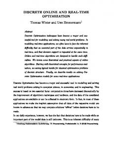
yk+N, uk+N Optimization Layer
Prediction of the Future Steady-State
yset ∆u
QDMC Regulatory Control Layer
uk
Process
yk
w Fig. 1. Two-layer strategy. dryer where a paste of homogenized chicken eggs is drying. Regulatory control and on-line search for optimum operational conditions are performed at the same frequency and in two steps (two-layer structure). The main differences are: (1) future stationary outputs and stationary control actions have both a different formulation and they are calculated from the inverse of the process gain matrix based on predictions upon a constrained QDMC controller and (2) no constraints are imposed in predict outputs, but only in set points, so a convex problem may be generated, which can be solved with less sophisticated optimization algorithms. The two-layer strategy is sketched in Figure 1. The two-layer optimization-control structure used in this paper was proposed by Schiavon Jr. (1998) and it follows the same idea of the proposed structure from Moro and Odloak (1995) with a few, but important modifications. The similarities among them are: (1) the optimization and regulatory control are performed in the same frequency and in two steps and (2) the future stationary outputs are predicted and supplied by a DMC controller.
2. FORMULATION OF THE STRATEGY In this structure, at each sampling time, the regulatory control and search for optimum operational conditions are performed at the same frequency and in two layers with strong interaction between them.
The new values of the manipulated variables, ? u, are supplied by the QDMC structure calculated from the following objective function
The Q − fr loop is closed using a PI (proportionalintegral) controller to maintain Q on its track. The
minΩ(∆u ) = (−A ⋅ ∆u + E′)T QTQ(−A ⋅ ∆u + E′) + ∆uT R∆u (1)
The production rate, Pr , is obtained by a semianalytical balance through the computer serial port RS232C. Another transducer measures bed pressure drop, ∆P . Polymeric capacitive meters measure air humidity in the outlet ( Ys ) and inlet ( Ye ). A
subject to the inequality constraints
∆u min ≤ ∆u ≤ ∆u max
(2)
(3) u min ≤ u ≤ u max Only the first value of ∆u calculated from equation (1) is implemented into the process and used to determine PN , which is required in the optimization layer. PN represents the effect from all last control actions over the future stationary outputs. Optimal set points are calculated from the following economical objective function
(
Φ y k + N , u k + N , ∆y
set
)
(4)
subject to the equality constraints y k + N = y k + PN + ∆ y set
(5)
1 set ∆y u k + N = uk + AN
(6)
temperature Ts is measured by a J-type thermocouple.
thyristor is employed to manipulate electrical power, POT . A diaphragm pump is used to regulate the feed flow rate of paste, Fe . All electrical signals, except for the balance and thermocouples, are of type 4-20mA standard protocol. These signals, including thermocouples, are sent to a Personal Computer through an AD/DA (analog/digital, digital/analog) interface. The spouted bed is built in steel and it has a conical cylindrical geometry (diameter = 15cm, air feed hole diameter = 3.5cm, height = 67.5cm, load height = 23.5cm, load = 3600g of glass particles as inert). Warm air is supplied with a flow rate in the range of 0 – 2.0 m3/min.
and also subject to the following inequality constraints set ∆y set ≤ ∆y set min ≤ ∆ y max
y set ≤ y set ≤ y set max min
(7) (8)
A convex problem is generated when the constraints are represented by equations (7) and (8). Observe that no constraints are imposed in predict outputs, but only in their set points. In this case the constraints do not change and the search domain will be always convex (there is not crossing of constraints which could eliminate the feasibility domain).
3. EXPERIMENTAL SET-UP Figure 2 sketches the experimental set-up used in all control implementations presented here. The spouted bed was assembled with several peripheral devices (including instruments) and a computer control. A motor frequency ( fr ) is manipulated to start and keep the spout. This frequency is applied in the blower's motor, which changes its speed rotation and, consequently, the air flow rate, Q . A frequency inverter is used to this purpose. The air flow rate Q is measured by a double orifice plate connected to a pressure transducer.
Fig. 2. Experimental system for the paste drying control in spouted bed. 1- spouted bed; 2- paste feed system; 3- cyclone; 4- air humidity sensor (capacitive); 5- thermocouple (J type); 6- pressure transducer; 7- power module (thyristor); 8electrical heat exchanger; 9- orifice plate flow meter; 10- blower; 11- psychrometer; 12frequency inverter; 13- PI controller; 14- signal conditioner; 15- PC AT-486 with A/D-D/A interface. The computer program for the experiments was written in C language and the sampling interval for acquisition and monitoring was 1s. The control algorithms were elaborated and tested in simulations using MATLAB before being implemented in C. The drying in the spouted bed was accomplished with the objective of obtaining powdered integral egg
with remaining moisture up to 5% in mass, under a temperature (at the bed exit) about Ts ≈ 70o C. It is possible to infer the product (powder) moisture contents ( X s ) from measurements of Ts and ( Ys − Ye ). This decision was made due to the high cost of an on-line humidity transducer for powders.
4. RESULTS FROM CLOSED-LOOP EXPERIMENTS The control objective of the two-layer real time optimization strategy is to maintain under control the exit temperature of the spouted bed dryer, Ts , and the difference between inlet and outlet air humidity ( Ys − Ye ). The manipulated variables are the feed flow rate of paste, Fe , and the electrical power supplied to heat the inlet air, POT . The economical objective function considered was a quadratic function of the power supplied to an electrical heat exchanger. The real time optimization solution sought to find the best operational conditions while the consumption of energy in the heater is minimized. Both, regulatory and economical optimization problems were solved by a QP algorithm. The control algorithm was written with Microsoft Quick C and it was implemented in a PC-type microcomputer. First, a 2 × 2 transfer function matrix was identified as a first order with time delay model, equation (9), based on experimental input step responses of Ts and ( Ys − Ye ), where time unit is given in minutes. Someone can argue that this is an inappropriate procedure nowadays. However, if you consider the difficulty of obtaining good models to predict the spouted bed behavior, the below proposed model, equation (9), seems to be fine. − 76 ⋅ e −0.8⋅ s T 19 ⋅ s + 1 s = (Ys − Ye ) 0.0320 ⋅ e − 0. 2⋅ s 1 ⋅ s + 1
23 .34 ⋅ e −2⋅ s 14 ⋅ s + 1 Fe ⋅ − 0.0014 ⋅ e− 9⋅ s POT 29 ⋅ s + 1
5% and another at t = 4700 s and magnitude of - 5%. In all cases, constraints were considered in all the manipulated and the set points of controlled variables. Tables 2 and 3 presents the upper and lower values considered for all these variables. The results from the first experiment, without disturbances, are showed in Figure 3. It displays that the real time optimization strategy was able to keep the controlled variables around the best operational conditions. The set points were gradually moved down to the lower bound constraints (Figures 3a e b). A decrease of the difference ( Ys − Ye ) of the moisture contents, represents a low consumption of energy demanded by the system. Therefore, the values of the set points for this variable, ( Ys − Ye ) set , were moved down in agreement with the economical objective, which indicates that the energy must be minimize (in fact
POT 2 is minimized, Figure 3e). In the same way, a small value of temperature, Ts , suggested that a small amount of energy is also supplied to the system, minimizing POT 2 (Figure 3a). Table 1 QDMC parameters Parameters N R L
Values 80 30 1
Parameters f α wpTs
Values 0.001 0 1
T
150
wp( Ys − Ye )
1000
Table 2 Bound constraints: first experiment Process Variables Fe (g/s)
Steadystate 0.25
Upper Value 0.35
Lower Value 0.15
POT (kW)
1.50 66
1.80 68.5
1.00 63.5
0.0035
0.0045
0.0025
Ts (9)
This model was used to calculate the convolution model (the dynamic matrix: A ) to perform the QDMC algorithm. Initial values of the QDMC parameters were estimated from simulation. Afterwards, the final values implemented were tuning from experimental tests. They are presented in Table 1. Two real time optimization tests were performed. In the first one (Figure 3), no disturbances were inputted in the process. In the second experimental test (Figure 4), some disturbances were accomplished in the feed flow rate of air ( Q ): one at t = 0 s and magnitude of +
set
0
( C)
( Ys − Ye ) set
Table 3 Bound constraints: second experiment Process Variables Fe (g/s)
Steadystate 0.25
Upper Value 0.35
Lower Value 0.15
POT (kW)
1.50 70
1.80 72.5
1.00 67.5
0.0035
0.0045
0.0025
Ts
set
0
( C)
( Ys − Ye ) set
outputs. And no violations of the set points occurred during the experiments.
set
Controlled variable (Ts)
66,0
Set-points (Ts ) Constraints
set
o
64,5 63,0 0
1000
2000
3000 4000 time (s)
5000
6000
7000
set
(YS-YE)
b) Controlled variable (YS -Y E) and Set-point (YS -YE ) x time 0,0042
Controlled variable (YS -YE )
0,0036
Set-point (Y S -YE ) Constraints
set
0,0030 0,0024 0
1000
2000
3000
4000 time (s)
5000
6000
7000
Fe (kg/seg.)x10
-3
c) Manipulated variable (Fe) x time 0,35 0,30
Manipulated variable Fe Constraints
0,25 0,20
1000
2000
3000
4000 time (s)
5000
6000
7000
d) Manipulated variable (POT) x time
1,8
POT (kW)
4b). Those oscillations were caused by the initial disturbance in the air feed flow rate. Approximately after 3000 seconds, the control system was able to compensate the effect of the disturbance and, then, the oscillations were finally reduced.
0,15 0
1,6 1,4
Manipulated variable POT Constraints
1,2 1,0 0
1000
2000
3000
4000
5000
6000
7000
2
time (s)
e) Economical function x time 2,5 2,0 1,5
POT
2
As in the first experiment, sometimes the output variables exceeded their set point constraints. This behavior may be also caused by model uncertainties during the prediction of future stationary state values. However, and in a similar manner, no violations occurred on input constraints. Excess of cool air during the first part of this second experiment helped the control system to move the temperature, Ts (Figure 4a), into its set point, faster than in the first experiment (Figure 3a).
1,0 0,5 0
1000
2000
3000
4000 time (s)
5000
6000
7000
Fig. 3. Two-layer structure without disturbances; economical objective is φ = minimize (POT2).
a) Controlled variable (Ts) and Set-Point (Ts ) x time
72
Controlled variable (Ts)
70
Set-points (Tsset) Constraints
68 66 0
Observe that the set points for this variable, Ts set , is
1000
2000
3000 4000 time (s)
5000
6000
7000
set
b) Controlled variable (ys-ye ) and Set-Point (ys-ye ) x time
(y s-y e)
depends basically on the feed flow rate of paste. Because a low amount of paste fed into the system will require more heating, a decrease in the feed flow rate of paste is not the best choice to control the temperature, Ts . However, it is also necessary to
-3
0,005
also decreased to its lower bound constraint. In this current experiment, the control of the temperature depends mostly on POT , while the control of the difference ( Ys − Ye ) of the moisture contents
0,004
Controlled variable (ys- ye)
0,003
Set-points (y s- ye)
set
0,002
Constraints
0,001
Fe (kg/seg.)x10
0
1000
2000
3000 4000 time (s)
5000
6000
7000
c) Manipulated variable (Fe) x time 0,35 0,30 0,25 0,20 0,15
Manipulated variable Fe Constraints
0
1000
2000
3000
4000 time (s)
5000
6000
7000
d) Manipulated variable (POT) x time
POT (kW)
control the difference of the mois ture contents. Manipulation of the electrical power supplied to heat the inlet air, POT , will not be just enough to control ( Ys − Ye ), which will demand an action of the feed
set
74
o
Economical function (kW)
The second experiment, now with disturbances in air feed flow rate, Q , is presented in Figure 4. It displays that the real time optimization algorithm was able to lead the controlled variables to their set points, although oscillations have been observed in the difference ( Ys − Ye ) of the moisture contents (Figure
Ts ( C)
Ts ( C)
a) Controlled variable (Ts) and Set-Point (Ts ) x time 69,0 67,5
1,8 1,6 1,4 1,2
Manipulated variable POT Constraints
1,0 0
1000
2000
3000 4000 time (s)
5000
6000
7000
6000
7000
Sometimes, the outputs variables did not track their set points accordingly. And they went beyond their desired values: the set point constraints (Figures 3a e b). However, no violations occurred on the inputs constraints (Figures 3c e d). This behavior of the output variables may be caused by uncertainties on the model used to predict the future stationary state, and not because of the real time optimization algorithm. Remember that, the optimization problem is subjected to constraints on set points and not on the
Economical function (kW)
2
flow rate of paste in this task.
e) Economical function x time
2,5 2,0 1,5
POT
2
1,0 0,5 0
1000
2000
3000
4000
5000
time (s)
Fig. 4. Two-layer structure with disturbance in the air feed flow rate; economical objective is φ = minimize (POT2).
5. CONCLUSIONS A good control performance was obtained in the experimental implementation of the two-layer real time optimization strategy. The algorithm was able to keep the controlled variables around the best operational conditions and to compensate the disturbances in air feed flow rate accordingly. However, sometimes the output variables exceeded their set point constraints, whose behavior can be caused by the model used to predict the future stationary state and not by the proposed control algorithm. Remember that the predicted outputs are not under constraints.
ACKNOWLEDGMENT Special thanks to CNPq (National Research Council of Brazil) and FAPESP (State of São Paulo Research Council) for the financial support to this project.
E′
Fe f fr L N PN POT
Pr Q
Q
R
R s T Ts u w
dynamic matrix matrix of stationary gains predict error vector based on the current and future control actions in the QDMC mass feed flow rate of paste suppression factor motor frequency control horizon model horizon vector of the steadystate effect of all past control actions electrical power supplied to inlet air production rate of dry powder weighting matrix for the predict errors in the QDMC volumetric feed flow rate of air weighted matrix for the control movements in the QDMC prediction horizon Laplace’s domain variable sampling period outlet air temperature manipulated variable disturbance
weight of Ts on Q
wp(YS −YE )
weight of ( Ys − Ye ) on Q outlet dry powder humidity inlet air humidity
Xs Ye Ys y Greek Symbols ∆P ∆u ∆y
Ω Φ Subscripts k k+N
GLOSSARY
A AN
wpTS
max min Superscripts set
outlet air humidity controlled variable
bed pressure drop control movement changing in the controlled variable QDMC objective function economical objective function
mmHg
present time future steady-state time upper value lower value
set point
g/s REFERENCES Hz
kW g/s
m3/min
s o C
Gouvêa, M. T., Odloak, D. (1998), One-layer real time optimization of LPG production in the FCC unit: procedure, advantages and disadvantages. Computers Chem. Engng. 22, Suppl., pp. 191198 Latour, P. R. (1979), Online computer optimization 2: benefits and implementation, Hydrocarbon Processing, 58, no. 7, pp. 219-223 Moro, L.F.L., Odloak, D. (1995), Constrained multivariable control of fluid catalytic cracking converters. Journal of Process Control, 5, no. 1, pp. 29-39 Odloak, D., Gouvêa, M. T. (1996), Control and optimization of a fluid catalytic cracking converter. Proceedings of the 1996 Brazilian Automation Congress (CBA), pp. 1411-1416. Schiavon Jr., A. L. (1998), Study of two real time optimization structures with QDMC, M.Sc. Thesis, Universidade Federal de São Carlos, São Carlos, Brazil (in Portuguese) Yousfi, C., Tournier, R. (1991), Steady state optimization inside model predictive control, Proceedings of the 1991 American Control Conference (ACC), pp.1866-1870