Two-level infinite mixture for multi-domain data
1 1.1
Simon Rogers Department of Computing Science University of Glasgow Glasgow, UK
[email protected]
Janne Sinkkonen and Arto Klami Department of Information and Computer Science Helsinki University of Technology Finland
[email protected]
Mark Girolami Department of Computing Science University of Glasgow Glasgow, UK
[email protected]
Samuel Kaski Department of Information and Computer Science Helsinki University of Technology Finland
[email protected]
Extended Abstract Introduction
The combined, unsupervised analysis of coupled data sources is an open problem in machine learning. A particularly important example from the biological domain is the analysis of mRNA and protein profiles derived from the same set of genes (either over time or under different conditions). Such analysis has the potential to provide a far more comprehensive picture of the mechanisms of transcription and translation than the individual analysis of the separate data sets. The problem is similar to that attacked with traditional Canonical Correlation Analysis (CCA) but in many application areas, the CCA assumptions are too restrictive. Probabilistic CCA [1] and kernel CCA [2] have both been recently proposed but the former is still limited to linear relationships and the latter compromises the interpretability in the original space. In this work, we preset a nonparametric model for coupled data that provides an interpretable description of the shared variability in the data (as well as that that isn’t shared) whilst being free of restrictive assumptions such as those found in CCA. The hierarchical model is built from two marginal mixtures (one for each representation - generalisation to three or more is straightforward). Each object will be assigned to one component in each marginal and the contingency table describing these joint assignments is assumed to have been generated by a mixture of tables with independent margins. This top-level mixture captures the shared variability whilst the marginal models are free to capture variation specific to the respective data sources. The number of components in all three mixtures is inferred from the data using a novel Dirichlet Process (DP) formulation.
1.2
The model
Each dataset consists of N instances, xn and y n . The marginal models are standard mixture models with components indexed by k (for x) and j (for y). The top level mixture is indexed by i. Using DP(α, H) to denote a Dirichlet Process with base measure H and concentration α, the model 1
follows the following specification Gx0 ∼ DP(γ x , H x ) ,
Gy0 ∼ DP(γ y , H y ) ,
Gxi ∼ DP(β x , Gx0 ) , π ∼ GEM(α) , θnx ∼ Gxzn ,
Gyi ∼ DP(β y , Gy0 ) , zn ∼ π , θny ∼ Gyzn ,
xn ∼ fx (x|θnx ) ,
y n ∼ fy (y|θny ) .
where the superscripts x and y in general denote the two margins, and GEM(α) is the stick-breaking distribution. Concentration parameters γ and β are margin-specific, defining the diversity, or “effective number” of the j (or k)-clusters, and α is the concentration parameter defining the diversity of the top-level clusters over i. Cluster parameters, originating from the base measures (priors) H x and H y , are denoted by θx and θy . Both margins have a hierarchy of DP’s [3], with the top-level processes Gx0 and Gy0 , and processes that are specific to the components i. The latent variables z are top-level cluster identities for the data samples. Finally, fx and fy are likelihoods of data, specific to each margin cluster j and k, but in the DP notation parameterized directly by the parameters sampled from the base measures and circulated through the DP hierarchies.
Hx
γx
βx
Gx0
Gxi
θnx
xn
θny
yn
zn Hy
Gy0
Gyi ∞
γy
N
βy
π
α
Figure 1: Mixture model plates diagram. Following the Chinese cuisine metaphor popular in models such as this, the Chinese restaurant franchise (describing the hierarchical DP model of [3]) has now grown from a finite to an infinite number of restaurants. Rather than customers being pre-allocated to restaurants, they are now allocated randomly, according to π. Unusually, each restaurant has two course-specific rooms (e.g., starter x and main course y) both with their own set of tables. As they must eat the correct course in each room, customers are assigned to one x-table and one y-table. The structures (Gx0 , Gy0 ) at the franchise headquarters and the local (Gxi , Gyi ) in restaurants exist for each course separately, and all decisions of the franchise are course-specific. The parameters α and γ describe how readily the franchise will open new restaurants and generate new dishes whilst β controls how keen the restaurants are to lay out new tables. This combination of multiple (here two) rooms of tables with room-specific dishes shared over an infinite number restaurants could be called Multi-Course Chinese Restaurant Franchise. 1.3
Estimation
We present a collapsed Gibbs sampler for sampling from the posterior distribution over assignments that is appropriate if the chosen DP base measures are conjugate to the likelihood. For a particular datapoint n, we first remove n from the current assignments and then assign it to a restaurant i (generating a new one if necessary) and then to marginal components, j and k, conditioned on this restaurant. Finally, dishes are re-assigned to tables and the various hyper-parameters are updated (unless fixed by the user). As in [4] (and described in more detail in [5]) it is also possible to treat 2
the various concentration parameters as random variables and sample them within the model. We use nested Metropolis-Hastings sub-samplers for this task but note that other alternatives are possible (e.g. [5]). 1.4
Synthetic Example
Whilst we have validated our model on both synthetic and real biological data, we will provide only synthetic results in this abstract. Figure 2(a) shows the two data sets with different symbols representing the true top-level grouping. The symbols are consistent across the two data sets. Therefore, there are three true top-level components, each of which comes from 2 marginal x components and one marginal y component. Multivariate Normal-inverse-Wishart priors were used for the marginal base measures (with hyper-parameters v0 = 3 (number of dimensions +1), κ0 = 1, µ0 = [0 0]T , Λ0 = [1 0; 0 1], see e.g. [6]) and Inverse-Gamma hyper-priors (p(α|a, b) ∝ α−(a+1) exp(−b/α)) were placed on each of the concentration parameters with hyper-hyperparameters a = b = 1. In Figure 2(b) we show the posterior distribution over top-level components (the inset plot shows the auto-correlation for this value) where it can be seen that the mode is positioned over the true value. The rather high weight given to I = 4 is predominantly due to the creation (and subsequent) destruction of singleton components. In the final plot, Figure 2(c), we depict the decomposition from a typical sample. For this particular sample, I = 3 and the top row shows the three contingency tables over the marginal assignments. From the size of these tables we can see that at this sample there were k = 4 components for x and j = 3 components for y. In the contingency tables, the lighter the color, the higher the probability (black = zero). Taking i = 1 as an example, we notice that the contingency table correctly picks out one y component and two x components, corresponding to the component depicted by blue squares in Figure 2(a).
References [1] Francis R. Bach and Michael I. Jordan. A probabilistic interpretation of canonical correlation analysis. Technical Report 688, Department of Statistics, University of California, Berkeley, 2005. [2] Alexei Vinokourov, John Shawe-Taylor, and Nello Cristianini. Inferring a semantic representation of text via cross-language correlation analysis. Advances in Neural Information Processing Systems, 15, 2002. [3] Yee Whye Teh, Michael I. Jordan, Matthew J. Beal, and David M. Blei. Hierarchical Dirichlet processes. Journal of the American Statistical Association, 101:1566–1581, 2006. [4] C. Rasmussen. The infinite Gaussian mixture model. In S. A. Solla, T. K. Leen, and K.-R. Muller, editors, Advances in Neural Information Processing Systems 12, pages 554–560. MIT Press, 2000. [5] M. West. Hyperparameter estimation in Dirichlet process mixtures. Technical Report 92-A03, Duke University, Institute of Statistics and Decision Sciences, 1992. [6] Andrew Gelman, John Carlin, Hal Stern, and Donald Rubin. Bayesian Data Analysis. Chapman and Hall, 2nd edition, 2004.
3
0.4 1
0.8
autocorrelation
0.3 p(I )
0.6
0.2
0.4
0.2
0.1
0
x
y
y-component
3
4
5
6 I
7
10
lag
8
20
9
x-component
(b) Marginal posterior distribution over the number of top-level components, I. (Inset - autocorrelation)
x-component
x-component
(a) Synthetic dataset for x (left) and y (right). Symbols/colors represent top-level clustering.
0 0
y-component
y-component
(c) Decomposition from typical sample. Top row shows contingency table mixture components (the lighter the color, the higher the probability) and bottom row shows data associated with this component. Notice how x and y are independent for each component alone.
Figure 2: Model results on synthetic data.
4