Online: http://www.parallax.com/detail.asp? product_id=BS2-IC, website of Parallax. Inc., developer and distributor of the Basic. Stamp 2 (BS2-IC) microcontroller ...
TWO-TANK LIQUID LEVEL CONTROL USING A BASIC STAMP MICROCONTROLLER AND A MATLAB-BASED DATA ACQUISITION AND CONTROL TOOLBOX Anshuman Panda,1 Hong Wong,2 Vikram Kapila,2 and Sang-Hoon Lee2 1
2
Department of Electrical and Computer Engineering Department of Mechanical, Aerospace, and Manufacturing Engineering Polytechnic University, Brooklyn, NY 11201 Introduction
A variety of PC-based data acquisition and control (DAC) boards are currently available in the market. These DAC boards can be broadly classified in two categories: i) high-end DAC boards, which provide a wide range of advanced hardware capabilities along with a sophisticated software environment, and ii) low-end DAC boards, which are primarily used for data acquisition of a few selective signals while using proprietary software. With the emergence of Matlab [1] as a widely used scientific computing tool in industry and academia, many users seek a DAC platform that can interface with and exploit advanced computing capabilities of Matlab to perform hardware in the loop experiments. Moreover, within the last decade, new developments in automated code generation programs have allowed users to utilize interactive icon-based control system simulation tools such as Simulink [2] for real-time control. In particular, using the Simulink block library and Real-TimeWorkshop (RTW) along with Simulink block libraries for vendor-specific DAC boards, one can generate C code from Simulink-based feedback control diagrams for real-time controller implementation on PC-based DAC boards. The ability to rapidly and efficiently design and implement complex control algorithms using an icon-based programming environment enables control designers to enhance productivity. Unfortunately, the use of Matlab as a software environment for DAC tasks frequently requires
the use of expensive DAC boards (over $1,000) which include advanced hardware features (e.g., high sampling rates and high resolution analog to digital converters) that a typical user may not utilize to the fullest potential. Thus, the use of existing PC-based DAC hardware and software solutions may be uneconomical for certain users (especially educators) interested in designing and building experiments that require a sophisticated software interface with minimal hardware costs. In contrast to the PC-based DAC boards, microcontrollers are inexpensive devices (costing only a few tens of dollars) which are widely used for embedded computing in hobby, academic, and industrial projects. However, a majority of microcontrollers require programming using one or other embedded programming variants of high-level programming languages (e.g., Basic, C, Java, etc.). In addition, many low-cost microcontrollers do not allow floating-point numerical computations that may be needed to implement advanced feedback control algorithms. In recent research [3], we have developed a low-cost DAC platform which allows microcontrollers to be programmed by Matlab and Simulink thus providing an inexpensive tool for data acquisition and control tasks. This platform is well suited for tasks that require graphical user interface and/or advanced computational capabilities, but do not require stringent hardware performance. It uses the advanced computing power of Matlab, the graphical user interface of Simulink, and
Parallax Inc.’s Basic Stamp 2 (BS2) microcontroller [4] to provide an environment which allows users to implement sophisticated control designs using inexpensive hardware. Furthermore, it provides a library of BS2 functions for Simulink, allowing for direct interaction between user-defined Simulink block diagrams and sensors/actuators connected to the BS2. The framework of reference [3] is significant for several reasons. First, it overcomes the two limitations common to most microcontrollers, viz., the lack of advanced icon-based software interface for efficient development of control algorithms and the lack of a graphical user interface (GUI) to allow intuitive interaction. In particular, our DAC toolbox overcomes these two limitations by extending the capabilities of Simulink to low-cost microcontrollers. Second, our DAC platform is very economical since it requires the use of only an off-the-shelf BS2 microcontroller (under $50) and obviates the need for overhead software such as RTW required for most PC-based DAC systems, thus further lowering the cost of acquiring such a system. This affords an opportunity to students to conduct industry-style rapid control prototyping and hardware in the loop experiments. Third, the ability to interface and program microcontrollers using the intuitive graphical programming environment of Simulink provides the flexibility and versatility of equipping a wide array of undergraduatelevel laboratories (physics, measurement systems, feedback control, and mechatronics) at an economical cost using our DAC platform. Fourth, our microcontroller-based DAC system is inherently portable due to its small size and low power requirement, extending its benefits to students who can acquire their personal DAC system for capstone design projects and for experimental research. In this paper, we illustrate several important features of the aforementioned DAC platform [3] by performing liquid level control of a coupled, two-tank system. Liquid level control is ubiquitous in industrial applications, e.g.,
food processing, effluent treatment, power generation plants, pharmaceutical industries, water purification systems, and industrial chemical processing. Thus, the study of liquid level control encompasses many engineering disciplines, e.g., electrical, chemical, civil, and mechanical. In this paper, we employ the classical proportional-plus-integral (PI) controller for liquid level control of a coupled, two tank system [5]. To effectively utilize this control methodology, the system parameters, e.g., tank dimensions and pump characteristics, must be known exactly. However, this may not be feasible since system parameters may change due to the effects of scaling in tanks and orifices, aging of pump, and wear. Thus, to determine the system parameters, we conduct an experimental system identification study which uses the inherent nonlinear dynamics of the two tank system. This paper is organized as follows. First, we outline the basic features of the Matlab data acquisition and control platform [3]. Next, we describe the coupled, two-tank system model and formulate system identification and control design objectives. Then we outline a method to perform system identification. In the next section we design a PI controller. Then we perform experimental validation of the results of earlier sections. Finally, we draw some concluding remarks. Matlab Data Acquisition and Control Platform In this section, we briefly outline the salient features of a software platform [3] that enables the use of an inexpensive microcontroller such as BS2 for data acquisition and control tasks. This framework allows Matlab and Simulink to seamlessly interact with the BS2 microcontroller; i.e., using the features of Simulink, this software platform allows for: i) automatic generation of PBasic code (the native programming language for the BS2 microcontroller) for a variety of sensors and
actuators that can be connected to the BS2 microcontroller; ii) programming of the BS2 microcontroller; and iii) data communication between the BS2 microcontroller and Matlab. In particular, this framework provides a library of Simulink functions, which allows for direct interaction between user-defined Simulink block diagrams and sensors/actuators connected to the BS2 microcontroller. See reference [3] for a detailed overview of this software platform.
an actuation signal, whose representation is in a digital format, to an analog output signal, we utilize the MAX537 digital to analog converter (D2A) IC, which is natively supported in the BS2 data acquisition and control toolbox. The MAX537 D2A IC is a 12-bit D2A and is manufactured by Dallas Semiconductor Inc. It can support up to 4 single output channels, which can be used as 2 differential outputs. For additional details on the MAX537 D2A IC, see website of Dallas Semiconductor [7].
Component Overview The PC-based data acquisition and control platform of reference [3] is composed of two main components, hardware and software. The hardware required for this platform is the BS2 microcontroller and user selectable sensors and actuators. The software required for this platform is Matlab with serial communication capability and Simulink. We refer to the software implementation of this PC-based data acquisition and control platform as the BS2 data acquisition and control toolbox. The BS2 microcontroller is used as a hardware interface that relays sensor data to and actuator data from a PC. Furthermore, the BS2 microcontroller communicates with the PC using a serial communication port. For further details on the BS2 microcontroller, see the Parallax website [4]. The BS2 data acquisition and control toolbox supports several different types of input and output signals (see reference [3] for a comprehensive list). However, in this paper, only analog input and output signals between ±5 Volts are considered. To convert an analog input signal to a digital format for use on a PC, we utilize the LTC1296 analog to digital converter (A2D) IC, which is natively supported in the BS2 data acquisition and control toolbox. The LTC1296 A2D IC is a 12-bit A2D and is manufactured by Linear Technology Inc. It can support up to 8 single input channels, which can be used as 4 differential inputs. For additional details on the LTC1296 A2D IC, see website of Linear Technology [6]. Analogously, to convert
Matlab is the primary software package used in the BS2 data acquisition and control toolbox. In addition to providing functionality for the Simulink toolbox, the Matlab scripting language allows for high level development of functions that can interface with specific hardware, in particular the serial communication port. Reference [3] exploits this capability by using built-in serial communication functions provided by Matlab (supported by versions 6.1 and higher) to communicate data with the BS2 microcontroller. Furthermore, the BS2 data acquisition and control toolbox utilizes the graphical user interface capabilities of Simulink to allow users to construct block diagrams interfacing with sensors and actuators. Simulink Block Diagram Design using BS2 Toolbox Overview The BS2 data acquisition and control toolbox allows users to implement control designs and to develop data acquisition and control panels within Simulink block diagrams. This toolbox provides a Simulink custom library, which contains blocks that interface with sensors and actuators connected to the BS2. See Figure 1 for a complete listing of sensor and actuator blocks currently available in the BS2 library. To use sensors and actuators available from the BS2 library, users must design a control panel or control algorithm using a predefined, blank, Simulink template model file. The key property of this template model file is the inclusion of functions used to program the BS2 microcontroller just before the Simulink block diagram is executed. When a user saves this
model file and runs the Simulink block diagram, a set of predefined operations are initiated before the Simulink block diagram is executed. These operations are as follows: i) define global variables to initiate serial communication; ii) generate PBasic code based on the sensor and actuator blocks used in the Simulink block diagram to be excuted on the BS2 microcontroller; iii) program the BS2 microcontroller via the serial communication port; and iv) start the Simulink block diagram if the BS2 microcontroller was successfully programmed, otherwise stop the block diagram and display an error message.
IOBlock: The main function of this block is to: i) initiate serial communication between the BS2 microcontroller and Matlab; ii) send and receive data between BS2 and Matlab; and iii) terminate this serial communication link. Aside from serial communication, another important task of IOBlock is to provide the sampling period of a given Simulink block diagram. This feature allows blocks that require the sampling period to be used properly, e.g., an integrator block or a timer block (clock). The sampling period is denoted as the amount of time required for one cycle of the Simulink block diagram to execute. The sampling period provided by the IOBlock is an averaged sampling period that is calculated by averaging the time taken to run a specified number of cycles of the Simulink block diagram. The number of cycles used for averaging is user definable, such that the user can adjust the resolution of the sampling period, i.e., a larger number of cycles will provide a finer resolution of the sampling period compared with a smaller number of cycles. However, this procedure of obtaining a sampling period does not provide the exact sampling period for each Simulink block cycle; thus, this BS2 data acquisition and control toolbox does not enforce any real-time requirements, i.e., enforcing a specific sampling period for the Simulink block diagram is not permissible. AtoD_LTC1296 block: This block receives voltage data from an LTC1296 A2D IC. The LTC1296 A2D IC is a 12-bit A2D (11-bit plus an additional sign bit) that has 8 single input channels, which can be used as 4 differential inputs. Furthermore, this IC is controlled by the BS2 via the serial peripheral interface (SPI).
Figure 1: BS2 Sensor and Actuator Block Library In this paper, we use only the blocks labeled IOBlock, AtoD_LTC1296, and DtoA_MAX537 from Figure 1. The following are brief descriptions of these blocks:
DtoA_MAX537 block: This block sends voltage data supplied by the Simulink block diagram to the MAX537 D2A IC. The MAX537 D2A IC is a 12-bit D2A (11-bit plus an additional sign bit) that has 4 single output channels, which can be used as 2 differential outputs. Furthermore, this IC is controlled by the BS2 via the serial peripheral interface (SPI).
Coupled Two-Tank System Model Figure 2 shows a two degree-of-freedom, state-coupled, two-tank system. This system consists of two tanks with orifices and liquid level sensors at the bottom of each tank, a pump, and a liquid basin. The two tanks have the same diameters and can be fitted with differing diameter outflow orifices. In this experimental setup, the pump provides the infeed to Tank 1 and the outflow of Tank 1 becomes the infeed to Tank 2. The outflow of Tank 2 is emptied into the liquid basin. The following conditions, with regard to the system dynamic model, are used to describe the levels of liquid in Tanks 1 and 2: i) the liquid level in Tanks 1 and 2, denoted as L1 (t ) and L2 (t ) , respectively, are measured using two pressure sensors; ii) L1 (t ) is always greater than 0 cm and less than 30 cm; iii) L2 (t ) is always greater than 0 cm; iv) the desired liquid level in Tank 2 is greater than 0 cm and less than 20 cm for t > 0 ; and v) the voltage applied at the input terminals of the pump, denoted by Vp (t ) , is between 0
Figure 2: Two Degree-of-Freedom, StateCoupled, Two-Tank System
and 22 Volts. The nonlinear mathematical model describing the liquid levels of Tanks 1 and 2 is given by [5] L�1 (t ) = − A L1 (t ) + BVp (t ), L� (t ) = C L (t ) − D L (t ) , 2
where A ∆=
1
2
(1) (2)
K a1 a 2 g , B ∆= p , C ∆= 1 2 g , and A1 A2 A1
a2 2 g , ai is the cross-sectional area of A2 the outflow orifice at the bottom of the Tank i , Ai is the cross-sectional area of the Tank i , K p D ∆=
is the pump constant, g is the gravitational acceleration, and i = 1, 2.
System Identification Objectives
In this paper, we assume that the system parameters A, B, C , and D or equivalently ai , Ai , K p , and g , for i = 1, 2, are not known exactly. As previously discussed, the uncertainty about system parameters may arise due to corrosive buildup in the liquid level system or the deterioration of the pump motor. Thus, a control design based on the idealized values of the system parameters may lead to performance deterioration for the closed-loop system. In a subsequent section, we outline a series of experiments, which exploit the nonlinear dynamics of (1) and (2), to numerically estimate the system parameters A, B, C , and D .
Control Objectives
Given a desired, constant, liquid level for Tank 2, denoted as L2 d , design a control input Vp (t )
Next, we develop the transfer function models for the linearized error system of (5)–(6) by taking the Laplace transform of (5) and (6) and rearranging terms to yield
such that lim L2 (t ) = L2 d . This objective is to be
A 1 ( s) β1 , = u ( s ) s − α1 β2 A 2 (s) = , A 1 ( s) s − α 2
t →∞
achieved with the assumption that L1 (t ) and L2 (t ) can be measured. Furthermore, the control design is to utilize estimates of the system parameters. To quantify this control objective, we define the liquid level tracking error for Tanks 1 and 2, i.e., A 1 (t ) and A 2 (t ) , as follows: A 1 (t ) ∆= L1 (t ) − L1d ,
A 2 (t ) ∆= L2 (t ) − L2d ,
(4)
In this section, we outline an experimental method to determine the parameters of the coupled two-tank system given in (1) and (2). Specifically, motivated by the nonlinear dynamics of (1) and (2), we outline a set of experiments that yield the system parameters A, B, C , and D . In experiment 1, we first obtain numerical values for the ratios A and C . In B D experiment 2, we obtain the numerical value for the parameter A , which using the numerical value of A obtained in experiment 1 yields B B . In experiment 3, we obtain the numerical value for the parameter D using the same procedure as in experiment 2, which using the numerical value of C obtained in experiment D 1 yields C .
⎛ a2 ⎞ ⎜⎜ ⎟⎟ L2d . ⎝ a1 ⎠
Linearized Error System Model
To facilitate the design of a controller to achieve the aforementioned control objectives, we begin by describing the linearized error system model (see reference [5] for details) A� 1 (t ) = α1A 1 (t ) + β1u (t ), A� 2 (t ) = α 2 A 2 (t ) + β 2A1 (t ),
(5) (6)
where u (t ) ∆= Vp (t ) − Vpd and Vpd is the desired pump voltage, which using (1) is characterized 2 gL1d as Vpd ∆= a1 . Furthermore, the parameters Kp
α1 , β1 , α 2 , and β 2 in (5)–(6) are defined as, respectively,
α1 ∆= − α
∆ 2 =
A , 4 L1d
β1 ∆= B ,
D , and β 2 − 4 L2d
∆ =
C . 4 L1d
where A 1 (s ) ∆= L [A 1 (t )] , A 2 (s ) ∆= L [A 2 (t )] , and u (s ) ∆= L [u (t )] with L denoting the Laplace operator [8]. System Identification
2
L
(9)
(3)
where L1d is some desired, constant liquid level for Tank 1, which using (2) is characterized as ∆ 1d =
(8)
(7)
Experiment 1
In this experiment, we obtain expressions that relate the ratios A and C to steady state B D conditions of the pump and the liquid level of Tanks 1 and 2. Specifically, we begin by noting that if a fixed voltage is applied to the pump, then the liquid level of Tanks 1 and 2 will reach steady state after a sufficient amount of time. This characteristic can be proven by directly solving the differential equations (1) and (2)
given that Vp (t ) is constant. Next, the solution of (1) and (2) under steady state conditions, i.e., with L�1 (t ) = 0 and L� 2 (t ) = 0, yields A Vpss , = B L1ss C = D
L2ss , L1ss
(10) (11)
respectively, where L1ss , L2ss , Vpss are the steady state liquid level of Tanks 1 and 2, and the steady state pump voltage, respectively. From (10) and (11), by applying a fixed voltage Vpss to the pump and directly measuring the liquid level of Tanks 1 and 2 after a sufficient amount of time, i.e., L1ss and L2ss , we can determine numerical values of A and C . B D
In this experiment, we fill Tank 1 with a fixed amount of liquid and record the time history of the liquid level in Tank 1 as it is discharged. Using this time history, we can determine a relationship between the system parameter A and the liquid level in Tank 1 at a given time instant. To do so, we solve the differential equation (1) with Vp (t ) = 0 and obtain 1 A(t − t0 ), 2
(12)
where t0 is the initial time and L1 (t0 ) is the initial liquid level in Tank 1. Note that equation (12) is only valid when the right hand side of (12) is nonnegative, i.e., prior to full discharge of Tank 1 since once Tank 1 is fully discharged the right hand side of (12) becomes negative. To determine when the liquid in Tank 1 is fully discharged, we set L1 (t ) = 0 in (12) and solve for the corresponding time, resulting in
2 L1 (t0 ) + t0 , A
(13)
where t * is the time of full discharge of Tank 1. Using (13), the analytic expression for the liquid level in Tank 1 is given by 2 ⎧⎛ 1 ⎞ ⎪⎜ L1 (t0 ) − A(t − t0 ) ⎟ 2 ⎪ ⎠ L1 (t ) = ⎨⎝ ⎪ 0 ⎪⎩
t