Using Control Theory to Achieve Service Level Objectives In Performance Management Sujay Parekh IBM
[email protected]
Neha Gandhi University of Michigan
[email protected] Dawn Tilbury University of Michigan
[email protected]
Joe Hellerstein IBM
[email protected]
Joe Bigus IBM
[email protected]
T. S. Jayram IBM
[email protected]
October 23, 2000 Abstract A widely used approach to achieving service level objectives for a target system (e.g., an email server) is to add a controller that manipulates the target system’s tuning parameters. We describe a methodology for designing such controllers for software systems that builds on classical control theory. The classical approach proceeds in two steps: system identification and controller design. In system identification, we construct mathematical models of the target system. Traditionally, this has been based on a first-principles approach, using detailed knowledge of the target system. Such models can be difficult to build, and too complex to validate, use, and maintain. In our methodology, a statistical (ARMA) model is fit to historical measurements of the target being controlled. These models are easier to obtain and use and allow us to apply control-theoretic design techniques to a larger class of systems. When applied to a Lotus Notes groupware server, we obtain model fits with R2 no lower than 75% and as high as 98%. In controller design, an analysis of the models leads to a controller that will achieve the service level objectives. We report on an analysis of a closed-loop system using an integral control law with Lotus Notes as the target. The objective is to maintain a reference queue length. Using rootlocus analysis from control theory, we are able to predict the occurrence (or absence) of controller-induced oscillations in the system’s response. Such oscillations are undesirable since they increase variability, thereby resulting in a failure to meet the service level objective. We implement this controller for a real Lotus Notes system, and observe a remarkable
1
correspondence between the behavior of the real system and the predictions of the analysis. This allows us to select the proper parameter for the controller from the analysis alone.
1
Introduction
Wide-spread reliance on IT systems has focused increasing attention on service level management, especially achieving response time and throughput objectives. A commonly used approach is to take an existing target system and add a controller that has access to the metrics and tuning parameters of the system. Based on the feedback information present in the metrics, the controller manipulates the tuning parameters to achieve the desired service level objectives. Examples of such closed-loop software systems abound: the network dispatcher [9, 8], which adjusts load balancing parameters in clusters of web servers; the Multiple Virtual Storage (MVS) workload manager [1], which adjusts memory allocations and other operating system tuning parameters to achieve response time and throughput objectives; and fair share schedulers [6], which adjust Unix nice tuning parameter to achieve fractional allocations of CPU. While considerable attention has been focused on the software mechanisms needed to enable closed-loop systems (e.g., instrumentation and tuning control access), much less attention has been paid to a rigorous evaluation of the behavior of the controller. Computer scientists most frequently use simulations to understand and evaluate controller behavior. However, simulation studies can be time-consuming, expensive, and error prone. The design of closed-loop or feedback control systems is also studied extensively in other engineering disciplines, such as mechanical and aeronautical engineering. In these engineering disciplines, designers most often employ linear control theory [15], which uses input-output relationships of linear systems to study controller properties such as: stability (finite inputs produces finite outputs), bias (how well objectives are achieved), rise time (how quickly the system responds to a change in objective), and settling time (how long until steady state is reached). This theory provides sound and rigorous mathematical principles for the design and analysis of closed-loop systems. The goal of our work is to develop a methodology for, and assess the value of, applying control theory to the evaluation of controllers used for service level management of software systems. While this is not a novel idea in itself, we believe that our approach enables the application of these techniques to a wider variety of systems than the traditional approach. In this paper, we also demonstrate the appeal and power of a control theoretic analysis on a controller for doing admission control of a Lotus Notes workgroup server. A primary concern with applying linear control theory to computer systems is that the assumption of a linear system is a poor fit to the realities of queueing in computer systems, which are highly non-linear. While there is a well-developed theory of non-linear control, it is much more difficult to apply,
2
does not generalize across systems and provides much less insight. Our perspective is more pragmatic. We pose the question “Can we construct and analyze the properties of real-life closed-loop software systems using the linear system assumption?” Even in mechanical engineering, a discipline where control theory is well-established, linearity often does not hold (e.g., turbulent fluid flows). Rather, the success of linear control theory has resulted from creativity in its application. The classical controller design methodology consists of two steps: System identification: Construct a transfer function which relates past and present input values to past and present output values. These transfer functions constitute a model of the system. Controller design: Based on properties of the transfer function and the desired objectives, a particular control law is chosen. Techniques from control theory are used to predict how the system will behave once the chosen controller is added to it. Previous work on the application of control theoretic techniques to computer systems ([5, 10, 14, 11, 17] to name a few) has generally used first principles to perform system identification. For example, the congestion control work typically constructs state transition equations based on detailed knowledge of (or assumptions about) the protocol, workload, losses, etc. Unfortunately, there are several short-comings with a first principles approach. First, for complex systems, it is difficult to construct a model from first principles, so often some unrealistic assumptions are made. This difficulty has been a major barrier to applying control theory to computer systems. Second, the first-principles models often employ detailed information about the target system. Since these details may change frequently (e.g., with each software release), a first-principles approach may require expert involvement on an on-going basis. This is expensive and often impractical. Third, the first-principles approach often does not address model validation. Without model validation, it is unclear how the insights obtained using control theory relate to the system being studied. Rather than proceeding from first principles, we advocate an empirical approach to system identification. Here, the input and output parameters need to be identified, just as before. But rather than deriving the transfer functions based on first-principles knowledge, an autoregressive, moving average (ARMA) model is constructed, and standard statistical techniques are employed to estimate the ARMA parameters. This approach treats the system as a black box, and thus is not affected by system complexity or lack of expert knowledge. Moreover, changes in the target system can easily be accommodated by re-estimating model parameters. In this paper, we show that the approach works well for the Notes server: R2 is no lower than 75%, and is as high as 98%. For the controller law, we use a saturated integral controller. The behavior of such a controller is determined by one parameter, called the gain. Control theory tells us that the gain should be large to obtain a fast response to changing inputs, but if it is too large, it can lead to undesirable behaviors in the system, 3
such as controller induced oscillations. The goal of the analysis, then, is to identify how large gain can be without causing these undesirable behavoirs. The particular form of the models allows us to use standard techniques from control theory to perform the analysis. Our results demonstrate that there is a remarkable correspondence between the predictions made by control theory and the observed behavior of an actual Notes server. In particular, we are able to identify the feasible gain values that satisfy the control objectives. The remainder of this paper is organized as follows. Section 2 describes the Notes server and how this target system is embedded into a closed-loop to achieve service level objectives. Section 3 details our approach to system identification. Section 4 discusses controller design and uses empirical studies to access the accuracy of insights obtained from control theory. We provide a summary and future work discussion in Section 5. Finally, Section 6 discusses related work.
2
Lotus Notes and Its Closed-Loop Control
This section describes relevant features of the Lotus Notes server and provides more details on how closed-loop control is obtained for this target system. Architecturally, Lotus Notes is a client-server system. Client software converts high-level user activity (mouse clicks, etc) into remote procedure calls (RPCs) that are sent to the server. The server maintains a queue of these inprogress RPCs. Once an RPC is serviced, an entry is made in the server log, and the appropriate response is sent to the client. Clients operate in a synchronous manner – waiting for the previous request to complete before sending a new request. The client/server protocol is session-oriented. An new session is begun after a session-initiating RPC is accepted by the server. We use the term offered load to refer to the load imposed on the server by client requests. In the case of homogeneous clients, offered load is expressed in terms of the number of clients. Our service level metric is the length of the queue of in-progress RPC requests, hereafter just referred to as queue length. The tuning parameter SERVER MAXUSERS regulates the number of users allowed to access the server at any time. This is a session-level control (as opposed to packet-level RPC controls). It operates by rejecting session-initiating RPCs once the number of connected users exceeds SERVER MAXUSERS. As such, this parameter has a somewhat complex effect on queue length. In particular, changing SERVER MAXUSERS has no effect until a session-initiating RPC arrives, so existing sessions are not affected. Unfortunately, we do not have direct measurements of RPC rates and queue length. Rather, we obtain these values from a measurement sensor that samples the server log at a rate of once a minute. The queue length computation is performed by counting RPCs that were active in the previous time quantum. However, since RPCs currently waiting in the queue are not present in the log, this approach underestimates the true queue length and true RPC rates. That is, measurement is lossy. We can improve the approximation by delaying one or
4
more time units before reporting the measurements since doing so allows more RPCs to complete and hence gives us a more accurate count of the RPCs that were executing.
Users RPCs
Reference value
Controller
Tuning control
Administrator
Sensor Server
Server Log
Queue Length
Figure 1: Closed-Loop Control of Lotus Notes Notes administrators are keenly interested in controlling queue length since this provides a way to manage trade-offs between response times and throughputs. Figure 1 shows how we construct a closed-loop system to control Notes queue length. Notes provides an interface for manipulating tuning parameters such as SERVER MAXUSERS. We use the measurement sensor described above to obtain values of queue length. The administrator specifies a desired value, or reference value, for queue length. The reference value specifies a management policy that the closed loop system tries to achieve. The controller takes as input the control error, which is the difference between the reference value and measured value of queue length. Depending on the current (and past) values of the error, SERVER MAXUSERS is adjusted. The algorithm that determines the value of SERVER MAXUSERS is called the control law.
3
System Identification and Validation
This section describes our approach to system identification and its application to Lotus Notes. System identification has three parts. The first, block diagram construction, identifies the significant functional components and their inputoutput relationships. The second, transfer function formulation, models the input-output relationships of each element in the block diagram. The particular form of the models we construct (linear transfer functions) is important because it enables us to leverage a large set of analysis techniques that are available in
5
control theory. The third, parameter estimation and evaluation, asseses the quality of the model developed.
3.1
Block Diagram Construction
A block diagram depicts the components of a system and the flow of information between them. Figure 1 provides a convenient starting point for modeling the Notes server. Here, RPC rates and SERVER MAXUSERS are inputs, and queue length is the output. This is depicted in Figure 2(a). RPC1 rate RPCn rate MaxUsers
Queue Length
Notes Server
(a) Initial Model
MaxUsers
Notes Actual Server Queue Length
Sensor
Measured Queue Length
(b) Final Model [Offered Load > Max_Users] Figure 2: Models of Notes server (open-loop) There are two problems with the foregoing. First, it is incomplete in that lossy measurements are not considered. Thus, a separate sensor component should be included. The second problem is more involved. Since SERVER MAXUSERS has an indirect effect on RPC rates, the two inputs are not independent. Hence this is not a linear system. To address this, we divide the operating region of the Notes server into two regions. In the first, SERVER MAXUSERS exceeds offered load and so the tuning parameter has no effect. In the second, SERVER MAXUSERS is lower than offered load and so exactly SERVER MAXUSERS users are allowed onto the system. We focus on the second operating region. Here, the offered load value is not relevant (as long as we stay in this region) and hence, it can be ignored. In other words, there is no need to consider RPC rates as an input. Can we adequately model the Notes server if SERVER MAXUSERS is the only input to the transfer function? To answer this question, Figure 3 plots queue length where the offered load is 300 users and SERVER MAXUSERS increased by 20 every 20 minutes. (These data are obtained using the experimental set up described in Section 4.4.) The impact of SERVER MAXUSERS is clear, suggest-
6
Offered load = 300 350
300
Queue Length, MaxUsers
250
200
150
100
Queue Length MaxUsers
50
0
0
0.5
1
1.5 Time
2
2.5 7
x 10
Figure 3: Effect of SERVER MAXUSERS on Queue Length ing that it would be sufficient. A more quantitative assessment is provided in Section 3.3. This results in the block diagram in Figure 2(b). Note that this is a singleinput, single-output system.
3.2
Transfer Function Formulation
We must now be more precise about quantifying input-output relationships. Throughout, we assume that time is discrete with uniform interval sizes. Consider a linear system with input x(t) and output y(t). By input-output relationships, we mean an autoregressive, moving average (ARMA) model of the form n m X X y(t) = ai y(t − i) + bj x(t − j) (1) i=1
j=0
where (n, m) is the order of the model, and the ai , bj are constants that are estimated from data. When values for n, m, ai , bi are specified, this is the transfer function of the linear system. For analysis purposes, it is much more convenient to convert the transfer functions from the time domain into the z (frequency) P∞ domain, where z is a complex number. That is, we want to use Y (z) = t=0 y(t)z −t , which is known as the z-transform. z-transforms have several nice properties. For example, consider two linear systems with transforms A(z) and B(z). Then the transform of the system
7
formed by connecting these two in series is A(z)B(z). If outputs of the two systems are summed, then the combined system has the transform A(z) + B(z). Also, if the input to A(z) is multiplied by k, then the associated transform is kA(z). Applying these principles to Eq. (1) and assuming that n ≥ m (which is a typical constraint), we obtain the z-transform: Pm n−j Y (z) j=0 bj z Pn (2) H(z) = = n X(z) z − ( i=1 ai z n−i ) We use the general form of the transfer function in Eq. (2) to determine N (z),the transfer function for the Notes-Server , and S(z), the transfer function of the Sensor component. Let q(t) be the value of queue length at time t and u(t) be the value of SERVER MAXUSERS. Note that this q(t) is the actual queue length, not the one produced by the Sensor. For N (z), it turns out that a good fit is obtained if n = 1 and m = 0 (see Table 1). That is, N (z) =
zb0 Q(z) = U (z) z − a1
This is a first order model since max(n, m) = 1. Modeling S(z) is a bit more involved. Let m(t) be the measured queue length as output by the Sensor. As discussed earlier, the Sensor output is lossy, so in general m(t) underestimates the real queue length q(t). Once again we use a first order model: m0 (t) = a1 m0 (t − 1) + b0 q(t) + b1 q(t − 1) whose transform is:
zb0 + b1 M0 (z) = Q(z) z − a1
However, this is not enough. Recall that to get an accurate estimate of q(t), we could delay d time units so that long-running RPCs present during time t complete their execution. To model this effect, define m(t) such that: m(t) = m0 (t − d). In the z-domain, this is simply z −d . Folding this into the previous equation, we obtain: S(z) =
M (z) zb0 + b1 = Q(z) (z − a1 )z d
Note that in modeling N (z) and S(z), we have treated the components as a black boxes, and have not used any details about their internal operation.
3.3
Parameter Estimation and Model Evaluation
Given the functional forms of N (z) and S(z), we must estimate their parameters. Our approach is statististical. First, measurements of the target system are 8
obtained while varying the input parameters in a controlled way, such as the data in Figure 3. Then, we use least-squares regression to estimate the ai , bj for different values of (n, m). In general the fit of the model improves as (n, m) are increased. We seek a model that has adequate fit and a low order. Delay All 0 1 2
Notes Server Sensor
R2 97.6 75.5 83.7 91.2
a1 0.4261 0.6371 0.7991 0.9237
b0 0.4709 0.1692 0.7182 0.9388
b1 0.0 -0.1057 -0.6564 -0.9092
Table 1: Model R2 Values and Coefficients How well do these transfer functions characterize the input-output relationships in the real system? One way to answer this question is to use the metric R2 , the fraction of the variability of the output variable that is explained by the transfer function. It turns out that a first order model provides a good fit for both N (z) and S(z). Table 1 reports values of the ai , bj and R2 for these transfer functions. For the Notes-Server, R2 is quite large, almost 98%! This is an excellent fit. The quality of this model can be further assessed by plotting observed values of queue length versus those predicted by the model, shown in Figure 4. Note that almost all observations lie close to the line of unit slope where the predicted value equals the actual value. 200 Data x=y
180
160
Predicted Queue Length
140
120
100
80
60
40
20
0
0
20
40
60
80 100 120 Observed Queue Length
140
160
180
200
Figure 4: Comparing N (z) model predictions with observed values For the Sensor transfer function, R2 is smaller, although still acceptable. Note that as d increases so does R2 , and a1 approaches 1. Both effects are expected since with longer delays, measured values approach the actual value.
9
4
Controller Design and Assessment
Having completed system identification, the next step is to design and assess one or more controllers. We begin by describing how to construct the controller from a control law. This is done under the assumption that the system is linear. Unfortunately, linearity does not always hold. Hence, a preliminary analysis is required to determine the conditions under which linearity is reasonable. We then use control theory to gain insights into controller behavior, especially the presence of controller induced oscillations. These predictions are assessed using measurements of a real Notes server.
4.1
Control Law and Closed-Loop Analysis
Control theory provides a systematic way to study feedback systems. Here, we show how to construct a transfer function of a closed loop system based on the transfer function of the target system in Figure 2(b). By constructing a closed loop system, we mean that the output of Figure 2(b) is fed back to the controller, which in turns compares this to the reference value r(t). Based on the difference between these two values, the controller computes a new setting u(t) for the control, which in our case is the value of SERVER MAXUSERS. This is shown in Figure 5.
R(z)
+ E(z) +
-
U(z)
G(z)
Controller
N(z)
Q(z)
Notes Server
S(z)
M(z)
Sensor
Figure 5: System with controller The starting point for controller design is a control law that describes how the controller operates. We focus on integral control [15], a widely used technique that is a reasonable approach for the Notes server. Only one control law is considered since our objective is to demonstrate the value of our methodology. A time-domain expression of the integral control law is u(t) = u(t − 1) + Ki e(t)
(3)
where u(t) is the new control value at time t, and e(t) = r(t)−m(t) is the control error. The parameter Ki > 0 is called the gain. Intuitively, this control law dictates that SERVER MAXUSERS be adjusted incrementally based on its previous value and the gain-weighted control error. From the definition of a transfer function, we have G(z) =
z U (z) = Ki = Ki D(z) E(z) z−1 10
(4)
For an integral controller, the intuition is that higher Ki values lead to a faster response. However, care is required since larger values of Ki can cause oscillations or even instabilities. There is a problem with directly translating this control law into software that is used for controlling Lotus Notes. Specifically, if |Ki e(t)| is too large, SERVER MAXUSERS is set to a value that can cause a software error. To avoid such situations, we limit the range of SERVER MAXUSERS by extending the control law: ∀t : M in ≤ u(t) ≤ M ax. Such saturated controllers are not linear. Thus, our modeling is restricted to regions in which these bounds are not reached. Using the principles of z-transforms discussed earlier, we have M (z) = E(z) =
E(z) ∗ Ki D(z)N (z)S(z) R(z) − M (z)
Solving these equations, we get the following transfer function for the system in Figure 5: M (z) Ki D(z)N (z)S(z) = (5) R(z) 1 + Ki D(z)N (z)S(z)
4.2
Preliminary Analysis
Since our model has been developed under the assumption that M in ≤ u(t) ≤ M ax, any analysis based on the model is necessarily restricted to this region as well. We peroform a preliminary analysis to determine the values of Ki for which this holds. Our approach is as follows. We divide the control region into three parts: u(t) = M ax, u(t) = M in and M ax < u(t) < M in. We designate these states as M ax, M in, and Intermediate, respectively. We seek to understand the conditions under which control values will be in states M in and M ax. If we stay away from these regions, then the assumptions of our analysis should hold. Figure 6 shows the state transitions obtained from the control law. We see that as Ki → ∞, all transitions are between states 1 and M ax. Clearly, we want to avoid large Ki . How big can Ki be without encountering states M in or M ax? Let be the largest error that occurs once the closed-loop system is in operation. Then, if M ax − M in Ki < we never transition into the extreme states. In our empirical studies of an uncontrolled Notes system, queue lengths range from approximately 20 to 100 if d = 0 and 60 to 140 if d = 2. So, if there is no bias, then in either case, = 40. We set M ax = 200 so that it equals offered load, and M in = 1. That gives us: Ki < 5.
4.3
Analytical Studies
This subsection uses classical control theory to evaluate the closed-loop system described by Eq. (5). We know from control theory that Ki should be as large 11
e >= 0
Max Min - Max