Type Elaboration and Subtype Completion for Java ... - CiteSeerX

Type Elaboration and Subtype Completion for Java Bytecode Todd B. Knoblock and Jakob Rehof November 23, 1999 Technical Report MSR-TR-99-79

Microsoft Research 1 Microsoft Way Redmond, WA 98052

Type Elaboration and Subtype Completion for Java Bytecode∗ Todd B. Knoblock and Jakob Rehof Microsoft Research MSR-TR-99-77 November, 1999

Abstract Java source code is strongly typed, but the translation from Java source to bytecode omits much of the type information originally contained within methods. Type elaboration is a technique for reconstructing strongly typed programs from incompletely typed bytecode by inferring types for local variables. There are situations where, technically, there are not enough types in the original type hierarchy to type a bytecode program. Subtype completion is a technique for adding necessary types to an arbitrary type hierarchy to make type elaboration possible for all verifiable Java bytecode. Type elaboration with subtype completion has been implemented as part of the Marmot Java compiler. 1

Introduction

Type elaboration is a technique for type inference on verifiable JavaTM bytecode. Verification provides type consistency rules that are based upon program flow and safety checking. These are weaker than the rules for static typechecking in Java source, and there are verifiable bytecode programs that are not typable under the Java typing rules. The central issue is that the type system of bytecode verification is based upon sets of types, and there may not be names for all of these sets in the Java type hierarchy. Subtype completion is a technique for adding a minimal number of new type names to make the bytecode typable. The present work was motivated by our goal of using a strongly typed intermediate representation as part of the Marmot bytecode to native code compiler [FKR+ ]. Strongly typed programming languages have long been recognized as improving program correctness and enhancing efficient implementation. More recently, it has been observed that type based intermediate representations and type ∗ This is an extended version of a paper published in Principles of Programming Languages, 2000 [KR00].

based compilation can extend these advantages to a compiler itself [Mor95, Tar96, LO98]. The use of types provides benefits in debugging the compiler, as well as in optimization and garbage collection. Many Java compilers use (or at least will accept) Java bytecode [LY99] instead of Java source programs as input [IBM98, Ins98, Nat98, Sup98]. However, some of the type information in the original Java source program is lost during the initial translation to bytecode. In order to use a typed intermediate representation, it is first necessary to reconstruct a strongly typed representation from the partially typed bytecode. The type system that we have chosen as the basis of our typed intermediate representation is a relatively simple one that has several advantages. First, it is very similar to the type system of Java. Second, it does not require sets of types representations, as does bytecode verification. Third, it is easy for a human to read, verify, and comprehend the typings. Fourth, it arises in a principled way from the (implicit) type system of bytecode verification. Finally, it is efficient to typecheck a program under this type system. Type elaboration is performed once, near the beginning the the compilation. After that, the fully typed program can be efficiently typechecked. In the standard mode of operation, the Marmot compiler will typecheck the program 10 times, and even on our largest benchmarks, each typecheck takes less than a second. During debugging, the system can perform dozens of typechecks in order to identify and isolate faults. In addition to its utility in type-directed compilation, type elaboration for bytecode solves a practical problem for Java decompilers such as Mocha that attempt to reconstruct Java source from Java bytecode. Once again, the simplicity of the underlying type system, and its similarity to the original Java type system, are advantages for this problem since the goal is to reconstruct the original program typings. In order to describe type elaboration, it is necessary that we examine three languages: Java source code, Java bytecode, and a typed intermediate rep-

Object

double float

Clonable

long int

Component ImageObserver ImageObserver[]

short

int[][]

char

Container[] Container

byte boolean

Null

Figure 1: Fragment of a Java type hierarchy. resentation that we refer to as the Java Intermediate Representation, JIR. These three languages have distinct, but related type systems. The Java source language has a traditionally defined type system presented as part of the standard language definition [GJS96]. Bytecode, per se, is untyped (or partially typed), but the rules for bytecode verification provide further consistency requirements based on dataflow and safety checking. Finally, the type system for JIR is closely related to the original type system for Java, and can be given a conventional set of typing rules. This paper investigates the formal relationship between these three typed languages and their type systems. Our main technical contributions are:

we return from the abstract problem to the concrete problem, and describe a number of other issues that must be addressed in implementing type elaboration, along with some comments on complexity and performance. Finally, we survey related work in section 8 and offer conclusions in section 9. 2

Types in Java bytecode

Java front-end compilers are responsible for translating Java source to bytecode. Java source code programs include complete static type information, but front-end compilers omit some of that information in the conversion to bytecode. The loss of type information in bytecode is apparent in several places:

1. We present a practical algorithm for type elaboration that accepts any verifiable bytecode.

• Local variables do not have type information.

2. We describe a technique called subtype completion, which transforms a subtyping system by conservatively extending its type hierarchy to a lattice. The technique is founded on the Dedekind-MacNeille completion, a mathematical technique for embedding a poset in a lattice.

• Evaluation stack locations are untyped. • Values represented as small integers (defined as booleans, bytes, shorts, chars, and integers) are convolved within bytecode methods. Separating the various types of small integers is especially useful because they are semantically distinct and valid in differing contexts. For example, while the representation of a boolean may be as another small integer type, boolean values should not be used in arithmetic expressions, and integer values should not be used where a boolean is expected. Although bytecode has lost some of the original typing of the Java source, nevertheless, much of the original type information from the program source has been preserved:

3. We formalize type-based safety checking present in Java bytecode verification. We show that subtype completion performed on a Javalike type system inserts exactly the extra types needed for verification, and it gives rise to a strongly typed intermediate representation (JIR) in a principled manner, together with a provably correct type inference algorithm. The paper is organized as follows. In sections 2 and 3, the types of bytecode, Java, and JIR are discussed. In sections 4 through 6, we present an abstraction of the problem and present the technical results on subtype completion. In section 7,

• All class fields maintain representations of the originally declared types.

2

Object interface SI { void siMeth(); } interface SJ { void sjMeth(); } interface I extends SI, SJ { ... }

SI

SJ

I

J

interface J extends SI, SJ { ... }

Null Figure 2: Type hierarchy representing multiple inheritance using interfaces. void foo(boolean flag, I i, J j) { if (flag) { x = i; } else { x = j; } x.siMeth(); x.sjMeth(); } Figure 3: Sample method that can not be typed in the given type hierarchy. • All function formals have types.

3

• The return value of a method, if any, has a type.

The type system of Java is defined, in part, by the widening conversions of the language [GJS96]. These encompass both the subtyping rules for reference types and the implicit coercions for numeric types. All of the widening conversions may be combined to form a partial ordering of the types of Java. We write A < B if there is a widening conversion from type A to type B. Figure 1 shows an example type hierarchy represented as a partial-order diagram.1 The type system of JIR is the same as that of Java except that all primitive numeric types are incomparable (i.e., there are no implicit, representation changing coercions) and the JIR system contains extra types in the subtype hierarchy. Type hierarchies for Java programs, as in other object-oriented languages, are partial orders, but not necessarily lattices. Figure 2 contains the outline of four interface definitions that give rise to the fragment of a type hierarchy shown. In this hierarchy, there is no least upper bound of I and J and

• Verified bytecode implies certain internal consistency in the use of types for locals and stack temporaries. What is missing is most of the type information within a method. The bytecode specification includes provisions for debug types on locals. This would appear to simplify at least part of the problem of elaboration. Unfortunately, (a) the debug types for locals are optional, (b) they do not distinguish between small integer types, (c) debug information is not available for the VM stack locations, and (d) they are frequently wrong or incomplete. Type elaboration assumes verified bytecode as input, but does not Bytecode verification assures various dynamic safety properties of the input program. It does not directly solve the problem of type elaboration because it does not distinguish between small integer types and handles multiple inheritance issues differently than the Java type system does.

The type systems of Java and JIR

1 In Java the type boolean may not be widened to any other type. However, to solve for the small integer types, it is useful to posit widening conversions for boolean for use within (and only during) type elaboration.

3

The language of J Local variables Parameters Field names Method names Constants

z x a f c

Expressions

e

LExpressions

le ::=

Statements

s

::=

le = e | returnf e | if(e) s1 else s2 | let z = e in s | s; s

Declarations

d

::=

f (x1 : τ1 , . . . , xn : τn ){s}

π ω τ σ

::= ::= ::=

null | . . . unit | ω | π τ | ω.τ | ~τ → τ ′

::=

c | x | z | e.a | f (e1 , . . . , en ) z | e.a

The Types of J Primitive types Reference types Base types (T0 ) Types (T ) Figure 4: Syntax of J and its types. code verifiers, that this step in verification requires that sets of types be employed. Moreover, the merge of the type states at the join point is the union of the possible types. Under this interpretation, the method in figure 3 is verifiable, but not typable in the given type hierarchy [Gol97, CGQ98, Qia98, Pus99, GH99].

no greatest lower bound of SI and SJ. Figure 3 contains a sample method (shown in pseudo-code rather than bytecode for clarity). The task for type elaboration is to solve for the type of local variable x relative to the type hierarchy in figure 2. We can see from the definitions of x that its type must be a supertype of both I and J, and further from the two uses, it must be a subtype of both SI and SJ. This method is an interesting case in bytecode verification. Verification defines the merging of two occurrences of a local variable at join points (such as the control point succeeding the if) as containing “an instance of the first common superclass of the two types” ([LY99] page 146). As has been noted by Qian, Goldberg, and others [Qia98, Gol97], it is not clear how this should be interpreted when the types in question are interfaces, especially when multiple inheritance is involved. 2 There appears to be general agreement, both in the work on formalizing Java bytecode verification, and in the actual implementations of byte-

4

An abstract type system for Java

In this section, we begin to study the problem of type elaboration in depth. We consider an abstract and simplified version of the problem which focuses on the core issue of how the three type systems (Java, bytecode, and JIR) are related. The typed language J is an abstraction of Java which captures the salient properties of the type elaboration problem. The syntax of the language J and its types are shown in Figure 4. The language J and its types The language J defined in Figure 4 includes method declarations with typed parameters and assignable local variables introduced in let-statements. The types of J (ranged over by σ) are built from base types (ranged over by τ ) which include the special type unit together with reference types (ranged over by ω) and primitive types (ranged over by π). Reference types include the special type null and object types. Primitive types include the boolean type and the numerical types of Java. Let T denote the set of all types, and let T0 denote the set of base types.

2

One strict reading of this language would have the first “superclass” of any interface be the Object type, as it is the only “class” that is a supertype of an interface. However, this reading would reject as unverifiable bytecode corresponding to legal Java programs. For example, consider having a method with a local declared as an Enumeration, an interface type, which is initialized as in one branch of a conditional as a VectorEnumeration, a class implementing an enumeration for a vector, and in the other branch of the conditional as a HashtableEnumeration. After the join, under the strict reading, this variable could not be used as an Enumeration, but only as an Object.

4

Expressions [ Cns ]

Σ; A ⊢ c : Σ(c)

[ Par ]

Σ(a) = ω.τ Σ; A ⊢ e : ω ′ ω′ ≤ ω [ Sel ] Σ; A ⊢ e.a : τ

Σ; A ⊢ x : Σ(x)

[ Var ]

Σ; A ⊢ z : A(z)

Σ(f ) = (τ1 , . . . , τn ) → τ Σ; A ⊢ ei : τi′ τi′ ≤ τi [ Inv ] Σ; A ⊢ f (e1 , . . . , en ) : τ

Statements Σ(f ) = ~τ → τ ′ Σ; A ⊢ e : τ ′′ τ ′′ ≤ τ ′ [ Ret ] Σ; A ⊢ returnf e : unit

Σ; A ⊢ le : τ Σ; A ⊢ e : τ ′ τ′ ≤ τ [ Asn ] Σ; A ⊢ le = e : unit Σ; A ⊢ e : τ Σ; A ⊢ s1 : unit Σ; A ⊢ s2 : unit τ ≤ boolean [ Cnd ] Σ; A ⊢ if(e) s1 else s2 : unit

Σ; A ⊢ e : τ Σ; A, z : τ ′ ⊢ s : unit τ ≤ τ′ [ Let ] Σ; A ⊢ let z = e in s : unit

Σ; A ⊢ s1 : unit Σ; A ⊢ s2 : unit [ Cmp ] Σ; A ⊢ s1 ; s2 : unit Declarations Σ(f ) = (ω, τ1 . . . , τn ) → τ ′ Σ(x) = ω ′ Σ(xi ) = τi , i = 1 . . . n Σ; A ⊢ s : unit ω′ ≤ ω [ Dcl ] Σ; A ⊢ f (x : ω ′ , x1 : τ1 , . . . , xn : τn ){s} : unit Figure 5: System J. Base types are assumed to be organized as a poset H = hT0 , ≤i, which defines a subtype or inheritance hierarchy. The expression form e.a is field selection. A field type is a pair ω.τ , where ω is an object type in which the field exists, and τ the type of the field itself. The form f (e1 , . . . , en ) is method invocation (e.f (e1 , . . . , en ) is written as f (e, e1 , . . . , en )), and method types have the form (ω, τ1 , . . . , τn ) → τ ′ , where ω is the type of the this-parameter. Local variables are introduced using let-statements of the form let z = e in s. Method definitions are accommodated by declarations f (x1 , . . . , xn ){s}, which define a method f with body s. A returnstatement is assumed to be tagged with the name of the method in whose declaration it occurs; any return statement in the declaration of method f

must have the form returnf e. A phrase, M , is either a statement, a declaration or an expression. Type system J The type system J is defined in Figure 5. These rules define derivable typing judgments of the form Σ; A ⊢ M : τ . The intended reading of such a judgment is that, under the typing assumptions given by the signature Σ and the type environment A, the phrase M has type τ . A signature is a function mapping field names, method names, parameters and constants to types. For M to be typable, all the field names, method names and constants occurring in M must be given types by Σ. The signature is intended to model declared types and the types of the basic constants of the language, which include predefined functions, such as arithmetic functions. It 5

F[[c]]

=

{Xc = Σ(c)}

F[[x]]

=

{Xx = Σ(x)}

F[[e.a]]

=

{Xe.a = τ } ∪ F [[e]] where Σ(a) = ω.τ

F[[f (e1 , . . . , en )]]

=

{Xf (e1 ,...,en ) = τ ′ } ∪ ( i=1 F[[ei ]]) where Σ(f ) = ~τ → τ ′

F[[z = e]]

=

{Xe ⊆ Xz } ∪ F [[e]]

F[[returnf e]]

=

F[[e]]

F[[if(e) s1 else s2 ]]

=

F[[e]] ∪ F [[s1 ]] ∪ F [[s2 ]]

F[[let z = e in s]]

=

{Xe ⊆ Xz } ∪ F [[e]] ∪ F [[s]]

F[[s1 ; s2 ]]

=

F[[s1 ]] ∪ F [[s2 ]]

F[[f (x : ω ′ , x1 : τ1 , . . . , xn : τn ){s}]]

=

{Xx = ω ′ } ∪ ( i=1 {Xxi = τi }) ∪ F [[s]] where Σ(f ) = (ω, τ1 , . . . , τn ) → τ ′ and Σ(x) = ω ′ , Σ(xi ) = τi , i = 1 . . . n

Sn

Sn

Figure 6: Type-flow constraints for system J. follows that only local (let-bound) variables have no declared types. A type environment, A, is a set of type assumptions of the form z : τ , which assigns type τ to local variable z. Only one assumption may occur for a given variable.3 The rules of Figure 5 are parametric in a given subtype hierarchy H and the signature Σ. We require that, whenever Σ(f ) = (ω, τ1 , . . . , τn ) → τ then ω is the largest type (with respect to H) such that f is a member of ω. We let J(Σ, H) denote the system obtained by using a specific hierarchy H and signature Σ in the rules for system J. The type inference problem for J is to reconstruct types for the local variables of a program in such a way that the program is well typed according to the rules of Figure 5. More precisely, given a phrase M , a signature Σ, and a hierarchy H, the type inference problem is to decide whether there exists a type τ and an assignment A of types to the locals of M such that Σ; A ⊢ M : τ . Note that because H can contain arbitrary finite subposets of interface hierarchies, the type inference problem for system J is NP-complete by reduction from satisfiability of inequalities over posets. The reduction follows from previous results on the complexity of subtype inference [LM92, Tiu92, PT96, Ben93, HM95], and a proof of NP-completeness for a framework similar to ours can be found in [GH99].

5

Bytecode verification

This section formalizes the relevant part of the rules of Java bytecode verification as they apply to our intermediate language J. It takes the form of a system of flow constraints generated from a program and a set of safety checking rules. The intention is that a program passes the verifier if and only if the safety checking rules are satisfied by the least solution to the flow-system generated from the program. 5.1

Flow system

The flow system shown in Figure 6 conservatively approximates the set of types of the values that a subexpression can evaluate to. The system of constraints generated from phrase M is denoted F[[M ]]. For the purpose of defining the flow system, we assume that each variable in the program has been renamed, so that the names are distinct. For each distinct occurrence of a subexpression e in the program, where e is not a local variable and not a parameter, the system uses a distinct flow variable named Xe to describe the possible types of e. Moreover, for each local variable z and each parameter x there will be a unique flow variable Xz , respectively Xx . Flow variables range over finite subsets of T0 . All constraints take the form Xe ⊆ Xe′ or Xe = τ . The latter form is a shorthand for Xe = {τ }.

3 In order to apply the present framework to a program, the program’s variables, field names, method names and parameters may have to be renamed appropriately. We tacitly assume that this has been done.

Lemma 5.1 For every phrase M , the constraint system F[[M ]] has a least solution.

6

(S1) For every occurrence of a subexpression of the form e.a: check that Xbe ⊑ ω, where Σ(a) = ω.τ

(S2) For every occurrence of a statement of the form e.a = e′ : check that Xbe′ ⊑ τ , where Σ(a) = ω.τ

(S3) For every occurrence of a subexpression of the form f (e1 , . . . , en ): check that Xbei ⊑ τi , where Σ(f ) = (τ1 , . . . , τn ) → τ ′

(S4) For every occurrence of a statement of the form returnf e: check that Xbe ⊑ τ ′ , where Σ(f ) = ~τ → τ ′

(S5) For every occurrence of a statement of the form if(e) s1 else s2 : check that Xbe ⊑ boolean

(S6) For every occurrence of a statement of the form f (x : ω ′ , x1 : τ1 , . . . , xn : τn ){s}: check that Xbx ⊑ ω, where Σ(f ) = (ω, τ1 , . . . , τn ) → τ ′

Figure 7: Verification rules for system J.

proof

5.2

See Appendix A.

from lattice theory [Mac37, Bir95, DP90]. Intuitively, this completion technique enriches the hierarchy H to a minimal lattice, by inserting missing least upper bounds and greatest lower bounds into H. Minimality means that the completion inserts new elements only where necessary. Other completion methods are known, such as ideal completion [DP90]. Moreover, the set-based flow-system of Section 5 is of course sufficient for verification. However, these methods introduce “unnecessary” elements. Consider a hierarchy P with types {⊥, A, B, C, D, ⊤}, ordered by x ≤ ⊤ and ⊥ ≤ x for all x in {A, B, C, D}. Ideal completion will include a distinct element for each of the 16 subsets of {A, B, C, D}. Each such element represents the least upper bound of the types in the subset. Flow-based safety checking may consider any subset of P . In contrast, Dedekind-MacNeille completion inserts no elements at all, since P is already a lattice and hence the minimal lattice containing itself. The result that type elaboration captures bytecode verification shows that, even though flowbased safety checking may consider many more sets than are produced by completion, the distinctions that can be made using these “extra” sets are irrelevant for safety.

2

Verification rules

For a given phrase M , let Xbe ⊆ T0 denote the meaning of flow variable Xe under the least solution to F[[M ]]. Then the verification rules for M are as defined in Figure 7. These rules use the notation S ⊑ τ , where S is a subset of T0 , defined by setting S ⊑ τ iff ∀τ ′ ∈ S. τ ′ ≤ τ . If the least solution to F[[M ]] satisfies the verification rules of Figure 7 using signature Σ and hierarchy H, then we say that M is safe with respect to Σ and H. Lemma 5.2 If M is typable in system J(Σ, H), then M is safe with respect to Σ and H. Note that verification accepts more programs than system J. Consider the method foo shown in Figure 3. It cannot be typed in System J, because the conditional requires x to have a type larger than both I and J, and the method invocations require x to have a type smaller than both SI and SJ; but no such type exists in the hierarchy shown in Figure 2. However, since Xbx = {I, J} holds for the least solution to F[[foo]], we have Xbx ⊑ SI and Xbx ⊑ SJ, and hence it is easy to see that foo satisfies the verification rules of Figure 7. 6

6.1

The Dedekind-MacNeille completion

Let hP, ≤i be an arbitrary poset. The DedekindMacNeille completion of P , denoted DM(P ), is the least complete lattice containing P as an isomorphic subposet. An order ideal is a downward closed subset of P , and the principal ideal generated from an element, x, is defined as ↓x = {y ∈ P | y ≤ x}. The poset P is contained in DM(P ) by the embedding x 7→↓x. In particular, DM(P ) preserves exist-

Subtype completion and the JIR type system

We will now show how the type system of JIR emerges by a completion of system J. The resulting JIR type system is a conservative extension of system J, which accepts exactly the verifiable (safe) programs. The construction is an application of the Dedekind-MacNeille completion known

7

Expressions [ Cns ]

[ Par ]

Σ; A ⊢ c : Σ(c)

[ Var ]

Σ; A ⊢ x : Σ(x)

Σ(a) = Ω.I Σ; A ⊢ e : Ω′ Ω′ ≤ Ω [ Sel ] Σ; A ⊢ e.a : I

Σ; A ⊢ z : A(z)

Σ(f ) = (I1 , . . . , In ) → I Σ; A ⊢ ei : Ii′ Ii′ ≤ Ii [ Inv ] Σ; A ⊢ f (e1 , . . . , en ) : I

Statements Σ; A ⊢ le : I Σ; A ⊢ e : I ′ I′ ≤ I [ Asn ] Σ; A ⊢ le = e : Unit

Σ(f ) = I~ → I ′ Σ; A ⊢ e : I ′′ I ′′ ≤ I ′ [ Ret ] Σ; A ⊢ returnf e : Unit

Σ; A ⊢ e : I Σ; A ⊢ s1 : Unit Σ; A ⊢ s2 : Unit I ≤ Boolean [ Cnd ] Σ; A ⊢ if(e) s1 else s2 : Unit

Σ; A ⊢ e : I Σ; A, z : I ′ ⊢ s : Unit I ≤ I′ [ Let ] Σ; A ⊢ let z = e in s : Unit

Σ; A ⊢ s1 : Unit Σ; A ⊢ s2 : Unit [ Cmp ] Σ; A ⊢ s1 ; s2 : Unit Declarations Σ(f ) = (Ω, I1 , . . . , In ) → I ′ Σ(x) = Ω′ Σ(xi ) = Ii , i = 1 . . . n Σ; A ⊢ s : Unit Ω′ ≤ Ω [ Dcl ] Σ; A ⊢ f (x : Ω′ , x1 : I1 , . . . , xn : In ){s} : Unit Figure 8: The JIR type system. ing joins and meets in P .4 We proceed to outline how DM(P ) is constructed from P . If A ⊆ P and x ∈ P we write x ≤ A if and only if x ≤ y for all y ∈ A, and we write A ≤ x if and only if y ≤ x for all y ∈ A. Define the sets Au and Aℓ as

by set inclusion. Meet and join in DM(P ) are given by

Au = {x ∈ P | A ≤ x} and Aℓ = {x ∈ P | x ≤ A}

where the operator C is as defined above. All elements of DM(P ) are order ideals, but not every ideal is an element of DM(P ).

^ i

Define the operator C by C(A) = Auℓ , then one has the basic properties A ⊆ C(A), A ⊆ B implies C(A) ⊆ C(B), and C(C(A)) = C(A). Now define the family of subsets DM(P ) by setting

6.2

Ai =

\ i

Ai and

_ i

[

Ai = C(

Ai )

(1)

i

The JIR type system

We now show how the type system of JIR arises from that of J(Σ, H) by applying the DedekindMacNeille completion to J. Its definition is given in Figure 8. Its base types are just the elements of DM(H), ranged over by I. We construct method types I~ → I ′ by setting

DM(P ) = {A ⊆ P | C(A) = A} that is, DM(P ) is the family of all subsets of P that are closed with respect to the operator C, ordered 4 Hence, if P is already a lattice, then DM acts as the identity, modulo isomorphism.

I~ → I ′ = {(τ1 , . . . , τn ) → τ ′ | τi ∈ Ii , τ ′ ∈ I ′ } 8

I[[c]]

=

{αc = Σ(c)}

I[[x]]

=

{αx = Σ(x)}

I[[e.a]]

=

{αe ≤ Ω, αe.a = I} ∪ I[[e]] where Σ(a) = Ω.I

I[[f (e1 , . . . , en )]]

=

′ {α Sfn(e1 ,...,en ) = I } ∪ ( i=1 I[[ei ]])∪ ( i=1 {αei ≤ Ii }) where Σ(f ) = (I1 , . . . , In ) → I ′

I[[le = e]]

=

{αe ≤ αle } ∪ I[[le]] ∪ I[[e]]

I[[returnf e]]

=

{αe ≤ I ′ } ∪ I[[e]] where Σ(f ) = I~ → I ′

I[[if(e) s1 else s2 ]]

=

{αe ≤ Boolean} ∪ I[[e]] ∪ I[[s1 ]] ∪ I[[s2 ]]

I[[let z = e in s]]

=

{αe ≤ αz } ∪ I[[e]] ∪ I[[s]]

I[[s1 ; s2 ]]

=

I[[s1 ]] ∪ I[[s2 ]]

I[[f (x : Ω′ , x1 : I1 , . . . , xn : In ){s}]]

=

′ {α Sxn = Ω , αx ≤ Ω}∪ ( i=1 {αxi = Ii }) ∪ I[[s]] where Σ(f ) = (Ω, I1 , . . . , In ) → I ′ and Σ(x) = Ω′ , Σ(xi ) = Ii , i = 1 . . . n

Sn

Figure 9: Type constraints for JIR. and, for a set Ω ∈ DM(H) consisting of object types and a base type element I we define the field type Ω.I by setting

6.3

Safety, typability and type inference

This section contains our main theoretical results on typability and type inference for JIR. We characterize the type inference problem for JIR, and show that the type system of JIR exactly captures the notion of safety of bytecode verification. Type elaboration for JIR reconstructs types for local (let-bound) variables. Type elaboration can be performed by solving a system of equalities and inequalities between types and type variables generated from the subexpressions of a given program, as specified in Figure 9. The constraint system generated from the phrase M is denoted I[[M ]]. Type variables α ∈ TyVar range over elements of DM(H). The constraint generation rules are given in terms of a signature Σ. Constraints take the form ξ ≤ ξ ′ , where ξ and ξ ′ are either a constant from DM(H) or a type variable, α. The following lemma records the fact that typability in the JIR type system is exactly captured by satisfiability of the constraint systems I[[M ]].

Ω.I = {ω.τ | ω ∈ Ω, τ ∈ I} We translate types σ of J to types dm(σ) of JIR by taking principal ideals of base types.5 We write Boolean = ↓ boolean and Unit = ↓ unit. A signature Σ is then translated to the signature DM(Σ) = dm ◦ Σ. The resulting system is denoted JIR(DM(Σ), DM(H)). The order relation in Figure 8 can be thought of in two (isomorphic) ways: as set inclusion, or as an extension of the order on H. It is useful to stress the latter view in the context of decompilation, where we desire typings that are as close as possible to the type system J. The completion DM(H) is instrumental to this by inserting only a minimal number of new points into H. In the example of figure 2, this amounts to inserting a new type, IJ, which is the least upper bound of I and J and the greatest lower bound of SI and SJ.

Lemma 6.1 A program M is typable in JIR(DM(Σ), DM(H)) if and only if the system I[[M ]] is satisfiable in DM(H). Moreover, every solution to I[[M ]] corresponds to a valid typing derivation in JIR(DM(Σ), DM(H)).

5

In detail, we let dm(τ ) = ↓ τ , dm(ω.τ ) = (↓ ω).(↓ τ ) and dm((τ1 , . . . , τn ) → τ ) = (↓τ1 , . . . , ↓τn ) → (↓τ ). Furthermore, we use the abbreviations Boolean = ↓ boolean, Unit = ↓unit and Null = ↓null.

proof The constraint system is a close reformulation of the typing rules. A detailed proof 9

can be constructed along the lines of Theorem 2.1 in [Wan87, KPS94], and is omitted. 2

on how type elaboration is implemented are given in Section 7. We will show one more property of DM(H) in the following lemma. It provides an optimization of the formula in Theorem 6.3, and it gives a succinct representation of the sets produced by completion. Whenever a set in DM(H) is isomorphic to an element in H, the representation gives back that element automatically. It is therefore the basis of “decompiling” the types of DM(H) back to the types of H. To state the lemma, we give a few definitions. For subsets A and B of H, we define the relation ⊑ by

Our next theorem establishes that the type system of JIR exactly captures the bytecode verification system defined in Section 5. The proof essentially consists of showing that the least solution to F[[M ]] can be translated to a minimal solution to I[[M ]], provided that M is safe, and, conversely that a minimal solution to I[[M ]] can be translated to the least solution to F[[M ]] such that the solution satisfies the verification rules. Theorem 6.2 (Soundness and completeness) A program M is typable in system JIR(DM(Σ), DM(H)) if and only if M is safe with respect to Σ and H. proof

See Appendix A for the proof.

A ⊑ B iff ∀x ∈ B. ∃y ∈ A. y ≤ x where the relation ≤ is the order relation of H. If A is a subset of H and x ∈ A, then x is called a minimal element of A iff y = x for any element y ∈ A with y ≤ x. Let Min A denote the set of minimal elements of A.

2

We now consider type inference. By Lemma 6.1, type inference for JIR reduces to solving type constraints over the lattice DM(H). Our next theorem characterizes the least solution to a satisfiable type constraint system. The theorem yields a low order polynomial type inference algorithm, and it is the foundation for the JIR type inference algorithm used in type elaboration. Note that all type constants in I[[M ]] are principal ideals, of the form ↓τ . To solve the constraints, it is not necessary to actually form these ideals, because we can represent a principal ideal, ↓τ , by its generator, τ . Accordingly, we define a translation ⌈•⌉ on types, given by ⌈↓τ ⌉ = τ , ⌈α⌉ = α, and we lift the translation to constraint sets C of the form I[[M ]] by defining ⌈C⌉ = {⌈τ ⌉ ≤ ⌈τ ′ ⌉ | τ ≤ τ ′ ∈ C}. If C = I[[M ]], and α is a variable in C, define the set Dα by setting

Lemma 6.4 Let A and B be subsets of the poset H. If H has no infinite descending chains, then one has Auℓ ⊆ B uℓ ⇔ Min (Au ) ⊑ Min (B u ) proof

φ−1 (Auℓ ) = τ ⇔ Min (Au ) = {τ }

Theorem 6.3 Let C = I[[M ]] and assume that C is satisfiable. Then there is a unique least solution µ to C in DM(H), which is given by

τ ∈Dα

proof

↑τ

!ℓ

See Appendix A for the proof.

(2)

(if Auℓ = ↓ τ , then Au = Auℓu = ↑ τ , hence Min (Au ) = {τ }; conversely, if Min (Au ) = {τ }, then Auℓ = {τ }ℓ = ↓τ .) This shows that the representation given by Lemma 6.4 automatically maps elements of DM(H) back to H, whenever this is possible. The application of Lemma 6.4 in type elaboration is discussed in more detail in Section 7.

where ⌈C⌉∗ is the transitive closure of ⌈C⌉.

µ(α) = (Dα )uℓ =

2

The previous lemma is applicable to solution sets of the form (Dα )uℓ from Theorem 6.3. The lemma shows that the function that maps a set of the form Auℓ to the set Min (Au ) is an order isomorphism.6 We can therefore represent (more efficiently) the operation •ℓ by the operation Min. Moreover, since φ(τ ) = ↓τ embeds H into DM(H), we know that

Dα = {τ ∈ H | τ ≤ α ∈ ⌈C⌉∗ }

\

See Appendix A for the proof.

7

Implementing type elaboration

Type elaboration has been implemented as part of the Marmot optimizing compiler [FKR+ ]. This section describes how type elaboration was implemented for the full Java bytecode. In addition to the issues formalized in the abstract system of the last few sections, a number of other, more pragmatic issues must be addressed, including that of typing small integer variables and the Java definition of covariant array subtyping.

2

Even though DM(H) may be exponentially large in the size of H, the solution formula in Theorem 6.3 only relies on types which are present in the constraint set. Therefore, solving a system I[[M ]] derived from a program M constructs only the types in DM(H) which are necessary for typing the particular program M . One can regard this as a kind of lazy completion, which avoids the exponential blow up; Theorem 6.3 gives rise to a polynomial time type inference algorithm. More details

6 This map is indeed a function: let f (X) = Min (X u ), for any X ⊆ H. Then f is a well defined function, and one has f (Auℓ ) = Min (Auℓu ) = Min (Au ), by the identity Auℓu = Au .

10

7.1

ble debug information) in the bytecode are assigned unique type variables of the form αn .

Preliminary processing

Because the stack-based bytecode is not a convenient compiler intermediate form for reasons beyond type elaboration, bytecode is first converted to a conventional temporary-variable based intermediate form, JIR. In JIR, references to the interpreter stack have been replaced by explicit temporaries which may be treated as normal local variables.7 It is legal in bytecode for a single local variable to hold values of distinct types at different places in the method. For example, local 3 may be used as both an int and as an Object within a single method. In verifiable bytecode, this is valid only if the lifetimes of the two uses of the local do not overlap (ignoring subroutines for the moment). Because type elaboration is required to assign a single type to each variable, it is necessary to separate any ambiguous uses of locals. This can be accomplished by renaming all uses of variables with distinct lifetimes. In Marmot, this is accomplished as a byproduct of converting to SSA form [CFR+ 89]. SSA form has the property that all static assignments to a variable have unique names. In the current example, the first name might become local 3’1 with type int and the second local 3’2 with type Object. Java bytecode includes instructions that support a form of light-weight subroutines which preserve the local variable context. Such subroutines may be used to represent the finally part of try/finally handlers. The verification rules for locals and their interactions with subroutines are complex. They allow, for example, multiple types for the same live local so long as that local is not referenced in the finally block. As Freund [Fre98] and O’Callahan [O’C99] have noted, the space savings from using bytecode subroutines does not appear to justify the substantial additional complexity. In Marmot, we chose to eliminate these subroutines by inline expansion. Type elaboration could be made to support subroutines directly, and in fact, we prototyped the code to support them, but eventually decided that the simpler expedient of inlining them was the more elegant solution. For the purposes of the following description of type elaboration, it is assumed that the bytecode input has been preprocessed such that all local variables and stack temporaries have been assigned designators, and all ambiguous uses with distinct lifetimes have been separated.

Step 1 Constraint collection Constraint collection proceeds on a per-method basis using constraint formation rules analogous to those given in figure 9. Equality constraints, x = y, are represented as two inequality constraints, x ≤ y and y ≤ x. For the purpose of constraint collection, small integer constants are given the type of the smallest containing small integer type. The signatures for phi applications, inserted as part of the translation to SSA form, are types of the from αn → α where n is the arity for the phi function, and α is a fresh type variable for each distinct phi. Step 2 Constraint closure Java defines covariant subtyping for array types: by definition A[] ≤ B[] iff A ≤ B for all reference types A and B. This rule requires that additional constraints be added to the constraint set in a process called constraint closure. Whenever a constraint is established between two potential array types, another constraint is induced between their element types. For example, if A[] ≤ B[] is established, then A ≤ B is also added to the constraint set. Further, recursively, if either A or B is a potential array type, then a constraint relating their element types is added. A potential array type is defined to be an explicit array type, A[] or a type variable, α that is related to (greater or less than or equal) to a potential array type. To relate a type variable’s element type to a potential array type, say A[], a fresh type variable is created and α = αelt [] is added to the constraints. Then A ≤ αelt or A ≥ αelt , as appropriate, is added to the constraint set. This in turn may require further closure on the constraint set. If a potential array eventually turns out not to be an array, then the type variable introduced as its “element” type is disregarded. The result of constraint collection and constraint closure is a finite set of constraints of the form A ≤ B, which relate types and type variables as employed in the program. The next task is to solve the constraints, that is to find an assignment of the types for all type variables such that the constraints are satisfied. Step 3 Cycle elimination

7.2

The type elaboration algorithm

Type elaboration first eliminates cycles in the constraint set by computing the strongly connected component of the constraints under the order relation [Tar72], and examines the acyclic directed hypergraph induced from the constraint graph by collapsing the nodes in a strongly connected component. All types within a strongly connected component are equal, and all type variables in it will

After preprocessing to JIR, all of the locals that did not have manifest types (either declared or credi7 While it is convenient to have unique names for variables during type elaboration, it would be possible to modify the type elaboration algorithms to work directly on the Java bytecode. Stack locations would be identified by both stack depth and program point.

11

Step 6 Applying the solution

receive the same assignment in the solution. The resulting graph is called the SCC graph and represents a partial order, the SCC order. The SCC graph is then traversed in depth-first order and the types in each strongly connected component are computed using theorem 6.3.

A final pragmatic issue is that it may not be possible to separate the uses of the small integers. A node in the SCC graph will normally contain at most one primitive type. For example, Object and Clonable would not be in the same SCC node in a verifiable program since they are distinct in the type hierarchy partial order. However, it is possible for small integer types, e.g., boolean and short to occur in the same node. This may happen because bytecode verification does not distinguish between these types and so bytecode may legally use a value of one small integer type where the another is expected (e.g., a short 1 as a boolean condition). This situation arises rarely in practice. When it does, all type calculations are based upon the join of the small integer types contained in the node. This is equivalent to equating, e.g., boolean and short, in the type hierarchy for the method being elaborated. To complete type elaboration, the solution is recorded for each type variable. Further, any implied widening conversions that involve representational changes (e.g., short to integer) are made manifest by inserting explicit coercions in the JIR. If the bytecode for a method convolves integer types in a way that causes a larger integer value to be used in a context expecting a smaller integer, then applying the solution will also introduce narrowing conversions for small integers. This is the only place where potentially unsafe narrowing conversions are introduced by type elaboration.

Step 4 Constructing filters In this step, order filters8 of the original type hierarchy are used in the construction of solution T types. This is done by computing the values τ ∈Dα ↑ τ for all variables α in the constraint graph, according to Theorem 6.3. Each such value is a subset of H. Note that the intersection of filters is a filter. The filters are computed incrementally by a single depth first traversal of the SCC graph, where the filter for each node is computed as follows: 1. If the node contains a base type, T , the solution type is the principal filter generated from T . The principal filters may be precomputed and cached for each source type. 2. If the node only contains type variables, the solution type is the intersection of the solution types of all immediate predecessors (lower elements in the SCC order). 3. The solution computed by the previous two steps is cached at each node, so that it can be used to incrementally compute the solutions for its immediate successors in the SCC order in 2.

7.3

Step 5 Constructing types

Complexity

As implemented in Marmot, in the worst case, the preprocessing of the bytecode (conversion to temporary form, lifetime splitting via SSA, and subroutine inlining) is exponential in the size of the original bytecode. It would suffice to implement preprocessing using a quadratic algorithm, resulting in a linear output.9 Let m represent the size of the program after preprocessing. Constraint collection (Step 1) takes time O(m) in the input size of the program (i.e., after preprocessing). Constraint closure (Step 2) takes time and results in a constraint graph that is O(d ∗ m) = O(m2 ) where d is the maximal depth of array type constructors. SCC formation (Step 3) is linear in the size of its input graph: O(d ∗ m) in this case. Calculating filters (Step 4) of lower bounds involves intersecting subsets of H. The sets are of size bounded by h, where h is the size of the hierarchy H. An intersection is performed at most once for each edge in the closed constraint graph. The intersections take time O(h)= O(m) per edge, hence O(d∗m∗h) in total. Precomputing the filters

In this step, we compute minimal elements of the filter intersections computed in step 4. This turns the filters computed in step 4 into types (isomorphic to those) of DM(H) and at the same time maps them back to H whenever possible. This step is founded on Lemma 6.4, which allows us to represent the value Aℓ by Min A, where A is a filter intersection. The type hierarchy H may have infinite descending chains due to the array type constructor: Object ≥ Object[] ≥ Object[][] ≥ . . . However, for any given program, the depth of array types will be bounded, and all descending chains will be finite for the section of H that matters for typing the given program. Lemma 6.4 is therefore applicable. 8 An order filter is an upward closed subset of a poset. The principal filter generated from an element x is denoted ↑x.

9 Subroutines may be supported using the jsr and ret instructions or encoded as in Freund [Fre98], and lifetime splitting without SSA conversion in O(n2 ) time and O(n) space where n is the size of the bytecode program.

12

100

Time (seconds)

10 1 0.1 0.01 0.001 0.0001 0.00001 1

10

100

1,000

10,000

100,000 1,000,000

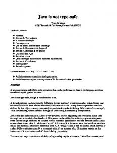
Method size (bytes) Figure 10: Per method type elaboration. relative to the size of the individual methods. Figure 10 shows the time it takes to type elaborate a method relative to the size of the unpreprocessed bytecode method. Note that the data is presented on a log-log scale, which makes the data for the very small method appear distinctly on the left of the graph. The data for this figure represents type elaboration run over approximately 22,300 methods from 65 programs.10 The methods range in size from 1 to 200,634 bytes. The largest method, a class initialization method written by an LALR parser-generator, took 18.5 seconds to type elaborate. Data was collected on an otherwise idle dual processor pentium II/300 Mhz processor computer running Windows NT/4. Type elaboration is run early in the optimization pipeline, and hence must solve types for many more methods and many more locals than will persist at later stages. Type elaboration times for entire benchmark programs range from 0.3 seconds to 45.5 seconds, representing approximately 4% of the compilation time. For comparison, SSA conversion represents approximately 5% of compilation time. Only 2 of the 65 programs had any methods that required that the small integer types be combined (one had 3 methods that convolved small integers, the other had 27 methods).

(represented as boolean vectors of length h) for all type constants requires O(h) calls to reachability in H (viewed as a graph) and hence is O(h2 ). The total cost of step 4 is therefore O(h2 + d ∗ m ∗ h) = O(m3 ). Constructing types (Step 5) by computing minimal elements of a set A ⊆ H can be done by processing the elements of A in reverse post-order: for each xi ∈ A taken in that order, we mark all unmarked nodes in H reachable from x in H. If xi is unmarked, we add it to the set Min A. This step visits an edge in H at most once (edges from marked nodes are not visited again), hence step 5 can be done in time O(h). Finally, applying the solution (Step 6) takes O(m) time. We have shown: Theorem 7.1 Let m be the size of the preprocessed program, let d be the maximal depth of array constructors in the program, and let h be the size of the hierarchy H. Then type elaboration can be computed in time O(h2 + d ∗ m ∗ h) = O(m3 ). Thus, the complexity of type elaboration excluding preprocessing is O(m3 ). If preprocessing were implemented using linear encoding of subroutines and variable lifetime splitting, then O(m)=O(n) and type elaboration takes O(n3 ) time, where n is the size of the original program. In practice, there is some evidence that the conversion to SSA and subroutine inlining are linear in the average case [CFR+ 89, Fre98]. Also, d and h will be small relative to n in most cases. 7.4

8

Related work

Gagnon and Hendren [GH99] also present an algorithm for type inference for Java bytecodes based upon solving constraints. Although superficially

Empirical Results

While the worst case complexity of type elaboration is in terms of the overall program size, it is interesting to examine the cost of type elaboration

10 There is some duplication of methods between the different programs caused, principally, by the runtime system.

13

similar, the approaches differ in important ways. Type elaboration successfully types verifiable bytecode that Gagnon and Hendren’s technique can not. Type elaboration is polynomial whereas their technique is exponential and type elaboration supports typing of the small integer types. Palsberg and O’Keefe [PO95] have shown that their notion of safety analysis is equivalent to typability in a subtyping system. A major difference to our results is that their type system is already lattice-based, so the problem of completion does not arise. Previous work, including [LM92, Tiu92, PT96, Ben93], has established that subtype inference over arbitrary posets is intractable. However, if the subtype order on base types is a lattice, the problem becomes PTIME solvable [Tiu92]. Subtype completion exploits this fact by transforming a poset to a lattice. The use of upward and downward closed sets, corresponding to order-filters and order-ideals of types is standard in many works on object-oriented analysis (e.g., [Bac97]). A¨it-Kaci et al. present data structures for efficient lattice operations on partially ordered sets representing inheritance hierarchies [ABLN89]. See also [Cas93], which describes an algorithm for lattice completion. There has been a substantial amount of work on formalizing various aspects of bytecode verification [Qia98, SA98, CGQ98, Yel99, Pus99, O’C99, Gol97]. Only a subset of these directly address the issue of verification with class hierarchies that have multiple inheritance. Others are focused on particular aspects of verification such as the polymorphism in subroutines [SA98, FM99, O’C99] or initialization of locals [FM98]. Goldberg [Gol97] and Qian [Qia99] formalize bytecode using dataflow and safety. Coglio et al. [CGQ98] formalize verification using constraints. A number of papers including [ON99, Sym97] have formalized the Java type system. League et al. [LST99] describe a typed intermediate language for Java based upon system F ω. Shivers [Shi91] presents a technique recovering what we called small integer types for Scheme. That domain is different, and more difficult, because the programs are not statically typed.

verification, allowing us to derive a provably correct type inference algorithm. In addition to issues caused by multiple inheritance, a practical implementation of type elaboration must work for verifiable bytecode that includes distinct variables assigned the same name, convolved small integer types, and the Java rule for covariant array subtyping. We have sketched how these pragmatic issues are addressed in the implementation of type elaboration in Marmot. Although the asymptotic complexity of type elaboration is cubic, it appears to be acceptable in practice. Type elaboration and the use of a strongly typed intermediate representation has proved to be a useful technique in the development of the Marmot compiler. Although having precise and accurate types is useful in optimization, the main benefit has been as a machine verifiable weak semantic correctness check used in debugging the optimizations. Of course, typechecking the intermediate representation can find only some errors in the compiler. The type system that we employ is relatively weak. By employing stronger type systems, it would be possible to catch a larger class of incorrect transformations [LST99, MWCG97, Nec98]. In addition to being too weak, the type system can also be too strong. A minor annoyance in employing a strongly typed intermediate representation is that, occasionally, one must augment optimization transformations so as to preserve typability of the intermediate representation. Even in the simple case of copy propagation, transformations must be inhibited in certain cases. For example, it is not legal to propagate a null constant into an array indexing context (because the element type is not explicitly stated). Nor is it legal to propagate a smaller array type into the left-hand-side of an array assignment replacing a larger array type (because of issues precipitated by the covariant array subtyping rules of Java). The technique of subtype completion can transform an intractable type inference system into a tractable one while preserving essential safety properties. This may be of independent interest beyond its application to type elaboration.

9

We would like to thank Erik Ruf, Bjarne Steensgaard, Bob Fitzgerald, and David Tarditi for ideas, implementation, and suggestions on improving the presentation.

Acknowledgements

Conclusion

This paper has presented type elaboration, a practical algorithm for recovering a strongly typed intermediate representation from partially typed verifiable bytecode. We showed that the type system of JIR arises in a principled way from the type system of Java and the flow-based verification of Java bytecode. For an abstract formalization of the problem, we showed that the technique of subtype completion adds just enough types to the subtype hierarchy to precisely correspond to the rules for bytecode

A A.1

Proofs Proof of Lemma 5.1

Before proving the lemma, we give a technical definition. For a system F[[M ]] of flow constraints (Figure 6), we divide its flow variables into two categories, typed and untyped. A flow variable Xe is

14

where Xet is a typed variable, and Xeu is an untyped variable (definitions of typed and untyped flow variables are given in Section A.1). We claim that φ solves the system F[[M ]] and satisfies all safety checks. Notice that all flow constraints in F[[M ]] have one of the forms Xet = τ or Xe ⊆ Xeu′ , where Xe is either typed or untyped. Since Max S ⊆ S, it follows that one has

called typed, if e is a formal parameter, a method invocation, a constant or a field selection. A flow variable is untyped if it is not typed. Lemma 5.1 For every phrase M , the constraint system F[[M ]] has a least solution. proof To see that any system of the form F[[M ]] has a least solution if it has any solutions, notice that the constraints in F[[M ]] have one of the forms X = τ or X ⊆ X ′ . Moreover, constraint variables range over sets of types, which form a lattice. Constraint resolution for systems of the form F[[M ]] therefore falls within the framework of monotone inequalities over a lattice, which implies the existence of least solutions to solvable constraint systems [RM99]. To see that every system F[[M ]] indeed has a solution, note, from the definition of F, that every constraint has the form X t = τ or Xe ⊆ X u , where Xe is either typed or untyped, X t is typed, and X u is untyped; moreover, whenever we have X t = τ1 and X t = τ2 then τ1 = τ2 . It then easily follows that every system can be solved by choosing sufficiently large sets of types for the untyped variables. 2 B

µ(αe ) ⊆ µ(αe′ ) ⇒ φ(Xe ) ⊆ φ(Xeu′ )

regardless of whether Xe is typed or untyped. We will use this observation freely in the following. We now show that φ solves F[[M ]] and satisfies all safety checks. We do so by considering all constraints generated from an arbitrary occurrence of a phrase in M . We consider each occurrence by cases over the form of the phrase, and for each such occurrence we consider the associated constraints and safety checks according to the definitions in Figure 6 and Figure 7: • Case f (e1 , . . . , en ) with constraint Xf (e1 ,...,en ) = τ ′ , where Σ(f ) = ~τ → τ ′ . The map φ solves the flow constraint: One has αf (e1 ,...,en ) = ↓ τ ′ in I[[M ]], and Xf (e1 ,...,en ) is typed. Hence, φ(Xf (e1 ,...,en ) ) = Max µ(αf (e1 ,...,en ) ) = Max (↓ τ ′ ) = {τ ′ }, as desired. The map φ satisfies the safety checks: The relevant safety check is (S3), requiring φ(Xei ) ⊑ τi . One has αei ≤ ↓τi in I[[M ]], hence µ(αei ) ⊆ ↓ τi , from which we get that µ(αei ) ⊑ τi , hence also Max µ(αei ) ⊑ τi , and therefore φ(Xei ) ⊑ τi , as desired.

Proof of Theorem 6.2

Theorem 6.2 (Soundness and completeness) A program M is typable in system JIR(DM(Σ), DM(H)) if and only if M is safe with respect to Σ and H. proof We begin by proving soundness, i.e., whenever M has a type in system JIR(DM(Σ), DM(H)), then M is safe with respect to Σ and H. To prove soundness, assume that M is typable, so that (by Lemma 6.1) we have a least solution µ : TyVar → DM(H) to the constraint system I[[M ]] (the fact that a least solution exists follows by an argument similar to the one given in the proof of Lemma 5.1). We now proceed to define a function φ (depending on µ), which maps flow variables to subsets of H. It will be shown that φ satisfies the constraints in F[[M ]] as well as all the safety checks of Figure 7. Soundness follows from the existence of φ with these properties, because if any one solution to F[[M ]] satisfies the safety checking rules, then so does the least solution to F[[M ]] (observe that all checks have the form S ⊑ τ , and if S satisfies this condition, then so does any subset of S). In order to define the map φ, let Max S denote the set of all maximal elements of the subset S ⊆ H (an element x ∈ S is maximal, if and only if x ≤ y implies x = y for all y ∈ S). The map φ : FlowVar → ℘(H) is then defined by φ(Xet ) φ(Xeu )

= =

(3)

• Case e.a, with constraint Xe.a = τ , where Σ(a) = ω.τ . One has DM(Σ)(a) = (↓ω).(↓τ ) and {αe ≤ ↓ ω, αe.a = ↓τ } ⊆ I[[M ]]. Therefore, µ(αe.a ) = ↓ τ . Since Xe.a is typed, one has φ(Xe.a ) = Max µ(αe.a ) = Max (↓τ ) = {τ }, so φ is seen to satisfy the flow constraint. The safety check requires φ(Xe ) ⊑ ω. Because αe ≤ ↓ ω is in I[[M ]], one has µ(αe ) ⊆ ↓ ω, and therefore µ(αe ) ⊑ ω. Because we have Max µ(αe ) ⊆ µ(αe ), it follows that φ(Xe ) ⊑ ω, as desired. • Case z = e with constraint Xe ⊆ Xz . We have αe ≤ αz in I[[M ]], so µ(αe ) ⊆ µ(αz ), hence φ(Xe ) ⊆ φ(Xz ). Here, we used that z is untyped, which guarantees that φ(Xz ) = µ(αz ), whereas φ(Xe ) is either µ(αe ) or Min µ(αe ), and the desired inclusion holds in both cases. There is no safety check associated with an assignment statement.

Max µ(αe ) µ(αe )

• Case x with constraint Xx = τ , where Σ(x) = τ . We have αx = ↓τ in I[[M ]], so that (using 15

the fact that Xx is typed) one gets φ(Xx ) = Max µ(αx ) = Max (↓τ ) = {τ }, as desired.

consider that the safety checking rules require that Xbe ⊑ ω, which implies Xbe ⊆ ↓ ω, and hence ψ(αe ) = (Xbe )uℓ ⊆ (↓ω)uℓ = ↓ω, as desired.

There is no safety check associated with a parameter occurrence. • Case f (x : ω ′ , x1 : τ1 , . . . , xn : τn ){s} with constraints Xx = ω ′ , Xxi = τi , where Σ(f ) = (ω, τ1 , . . . , τn ) → τ ′ .

• Case z = e with constraint αe ≤ αz .

One has Xe ⊆ Xz in F[[M ]], hence Xbe ⊆ Xbz , hence (Xbe )uℓ ⊆ (Xbz )uℓ , which shows that ψ(αe ) ⊆ ψ(αz ), as desired.

One has {αx = ↓ω ′ , αx ≤ ↓ω, αxi = ↓τi } ⊆ I[[M ]], and Xx and Xxi are all typed. It follows that one has φ(Xx ) = Max µ(αx ) = Max(↓ω ′ ) = {ω ′ } and φ(Xxi ) = Max µ(αxi ) = Max (↓τi ) = {τi }, and the flow constraints are seen to be satisfied under φ.

• Case e.a = e′ with constraint αe′ ≤ αe.a , where Σ(a) = ω.τ . One has Xbe.a = τ by the constraints in F[[M ]], and moreover Xbe′ ⊑ τ by the safety checking rule (S2). It follows from the former relation that ψ(αe.a ) = {τ }uℓ = ↓τ , and since Xbe′ ⊑ τ , we get Xbe′ ⊆ ↓ τ , which implies ψ(αe′ ) ⊆ ↓ τ = ψ(αe.a ). This shows that ψ satisfies the inequality generated in this case.

The safety rules require φ(Xx ) ⊑ ω. Since we have αx ≤ ↓ ω in I[[M ]], it follows that φ(Xx ) = Max µ(αx ) ⊆ µ(αx ) ⊆ ↓ω, and therefore φ(Xx ) ⊑ ω, as desired. The remaining cases are similar and left out. This concludes the soundness proof. To prove completeness, we need to show that, whenever the least solution to F[[M ]] satisfies the safety checking rules of Figure 7, then the constraint system I[[M ]] has a solution in DM(H), so that (by Lemma 6.1) M types. We will do this by defining a mapping ψ from type variables to DM(H) depending on the least solution to F[[M ]]. The function ψ : TyVar → DM(H) is defined by

• Case x with constraint αx = ↓τ , where Σ(x) = τ. By the definition of F[[M ]], one has Xbx = τ , and therefore ψ(αx ) = {τ }uℓ = ↓τ , showing that ψ satisfies the inequality in this case. • Case f (x : ω ′ , x1 : τ1 , . . . , xn : τn ){s} with constraints αx = ↓ ω ′ , αx ≤ ω, αxi = ↓ τi , where Σ(f ) = (ω, τ1 , . . . , τn ) → τ ′ .

ψ(αe ) = (Xbe )uℓ

One has Xbx = ω ′ and Xbxi = τi by the definition of F[[M ]]. These relations imply that ψ(αx ) = ↓ω ′ and ψ(αxi ) = ↓τi . Moreover, by the safety check (S6), we know that Xbx ⊑ ω, so that Xbx ⊆ ↓ω, hence ψ(αx ) ⊆ ↓ω, and all constraints are seen to be satisified under ψ, as desired.

We show that all constraints generated from an arbitrary occurrence of a phrase in M are satisfied under the mapping ψ, provided that the least solution to F[[M ]] satisfies all safety checks. We proceed by cases over the form of phrases: with constraints • Case f (e1 , . . . , en ) αf (e1 ,...,en ) = ↓ τ ′ , αei ≤ ↓ τi , where Σ(f ) = (τ1 , . . . , τn ) → τ ′ .

The remaining cases are similar. This concludes the proof of completeness. 2

One has Xf (e1 ,...,en ) = τ ′ in F[[M ]], so that Xbf (e1 ,...,en ) = {τ ′ } holds, and therefore we have ψ(αf (e1 ,...,en ) ) = {τ ′ }uℓ = (↑τ ′ )ℓ = ↓τ ′ , which shows that ψ(αf (e1 ,...,en ) ) ⊆ ↓ τ ′ , and so ψ solves the first type inequality mentioned above. To see that the second inequality is also satisfied under ψ, consider that the safety check (S3) requires that Xbei ⊑ τi . It follows that Xbei ⊆ ↓ τi , and therefore one has ψ(αei ) = (Xbei )uℓ ⊆ (↓ τi )uℓ = ↓ τi , thereby showing ψ(αei ) ⊆ ↓τi , as desired.

B.1

Proof of Theorem 6.3

In order to prove Theorem 6.3 we need to understand the satisfiability problem for inequalities over the lattice DM(H). Here it is useful to look at an abstract version of the problem first, by recalling a general lemma concerning inequalities over an arbitrary complete lattice. In order to state this lemma, we need a few definitions. Let P be any poset. A system of inequalities over P is a finite set of formal inequalities of the form α ≤ α′ , k ≤ α or α ≤ k, where α and α′ range over variables and k ranges over constants drawn from P . A system C is said to be satisfiable in P if and only if there exists a substitution v from variables to elements of P such that v(ξ) ≤P v(ξ ′ ) is true in P , for all ξ ≤ ξ ′ ∈ C (here ξ and ξ ′ range over variables or constants from C). The closure of a system C, denoted C ∗ , is the least

• Case e.a with constraints αe ≤ ↓ω, αe.a = ↓τ , where Σ(a) = ω.τ .

One has Xe.a = τ in F[[M ]], hence Xbe.a = {τ }, and hence ψ(αe.a ) = {τ }uℓ = ↓ τ , proving that ψ satisfies the constraint αe.a = ↓τ . To see that ψ satisfies the constraint αe ≤ ↓ ω, 16

T

system of inequalities containing C and satisfying the condition (ξ ≤ ξ ′ ) ∈ C ∗ , (ξ ′ ≤ ξ ′′ ) ∈ C ∗ ⇒ (ξ ≤ ξ ′′ ) ∈ C ∗ A system C is said to be consistent if and only if we have (k1 ≤ k2 ) ∈ C ∗ ⇒ k1 ≤P k2

S

for all k1 , k2 ∈ P . Finally, for a system of inequalities, C, define for each variable α in C the subset ↓C (α) ⊆ P , given by

Then we have Lemma B.1 Let L be a complete lattice, and let C be a system of inequalities over L. Then C is satisfiable if and only if C is consistent. Moreover, if C is satisfiable, then the substitution µ given by µ(α) =

x∈

B.2

↓C (α)

proof It is standard that the substitution µ solves C, whenever C is consistent, and proofs of this fact in a subtyping setting can be found in, e.g., [LM92, Tiu92]. It is easy to verify that µ must be the least solution to C, if indeed µ is a solution. 2

=

τ ∈Dα

↑τ

_

↓C (α)

!ℓ

proof

Easy.

2

(⇒). One has

by the identity Auℓu = Au and anti-monotonicity (with respect to inclusion) of the operations •u and •ℓ . Now, B u ⊆ Au implies Au ⊑ B u , by Lemma B.2, which is applicable since Au and B u are upward closed sets. (⇐). Assume Au ⊑ B u . Since •ℓ is antimonotonic with respect to inclusion, it is sufficient to show that B u ⊆ Au . So let x ∈ B u . Then, by the assumption, Au ⊑ B u , there exists y ∈ Au with y ≤ x. Since Au is upwards closed and y ∈ Au and y ≤ x, it follows that x ∈ Au . We have shown 2 B u ⊆ Au as desired.

↓C (α)

W W{↓τ | ↓τ ∈↓C (α)} W{↓τ | τ ∈↓⌈C⌉ (α)} ↓τ
uℓ Sτ ∈Dα ↓τ = τ ∈Dα
ℓ T = (↓τ )u τ ∈Dα
ℓ T τ ∈Dα

2

Auℓ ⊆ B uℓ ⇒ (B uℓ )u ⊆ (Auℓ )u ⇔ B u ⊆ Au

= = =

=

.

Lemma B.3 Let A, B be subsets of a poset P . Then Auℓ ⊆ B uℓ ⇔ Au ⊑ B u

with C = SI[[M ]]. Now recall that we have W uℓ A = ( A ) , by equation (1). Moreover, i i i∈I i∈I itSis easy to verify, using definitions, that one has T ( i∈I Ai )u = i∈I (Ai )u and (↓ x)u =↑ x. Using these identities, we can compute as follows:

W


u

Proof of Lemma 6.4

proof

proof We apply Lemma B.1 to the case L = DM(H), which allows us to characterize the least solution µ to I[[M ]] by µ(α) =

↓τ

A⊆B⇔B⊑A

Theorem 6.3 Let C = I[[M ]], and assume that C is satisfiable. Then there is a unique least solution µ to C in DM(H), which is given by µ(α) = (Dα )

τ ∈Dα

Lemma B.2 Let A and B be upward closed subsets of a poset P . Then

To prove Theorem 6.3, recall the definition of Dα , Dα = {τ ∈ H | τ ≤ α ∈ ⌈C⌉∗ }

\

S

In order to prove Lemma 6.4 we first prove a couple of auxiliary lemmas. Recall that we define A ⊑ B by A ⊑ B iff ∀x ∈ B. ∃y ∈ A. y ≤ x

is the least solution to C.

uℓ


u

↓τ . Then to left, suppose that x ∈ τS ∈Dα S x ≥ τ ∈Dα ↓ τ . Since Dα ⊆ τ ∈Dα ↓ τ , it follows that x ≥ Dα , hence x ∈ (Dα )u . To see the other inclusion, assume x ∈ (Dα )u . Then for any y ∈ Dα one has x ≥ y. HenceSx ≥ ↓ y for all y ∈ Dα , and therefore also x ≥ τ ∈Dα ↓τ , hence

↓C (α) = {k ∈ P | (k ≤ α) ∈ C ∗ }

_


ℓ

↑τ solves C. which proves that µ(α) = τ ∈Dα At the first equation in the calculation above we used the fact that the only constants occurring in constraint systems of the form I[[M ]] are principal ideals, of the form ↓τ .
ℓ T ↑τ , it is suffiTo see that (Dα )uℓ = τ ∈Dα cient equations) to show that (Dα )u =
u S (by previous ↓τ . To see the inclusion from right τ ∈Dα

Lemma B.4 Let A and B be subsets of the poset H. If H has no infinite descending chains, then one has A ⊑ B ⇔ Min A ⊑ Min B

↑τ

17

proof (⇒). Assume A ⊑ B. Let x ∈ Min B. Then, by the assumption, there is y ∈ A such that y ≤ x. Since H has no infinite descending chains, we can find ym ∈ Min A such that ym ≤ y. So we have ym ≤ x, hence we have shown MinA ⊑ MinB. (⇐) Assume Min A ⊑ Min B. Let x ∈ B. Then, since H has no infinite descending chains, we can find xm ∈ Min B such that xm ≤ x. Then, by the assumption, there is y ∈ Min A such that y ≤ xm , hence also y ≤ x. This shows that A ⊑ B. 2

[CGQ98]

Alessandro Coglio, Allen Goldberg, and Zhenyu Qian. Towards a provably-correct implementation of the JVM bytecode verifier. Technical Report KES.U.98.5, Kestrel Institue, August 1998 1998. Also availabe in Proceedings of the OOPSLA ’98 Workshop on the Formal Underpinnings of Java, Vancouver, B.C., October 1998.

Lemma 6.4 Let A and B be subsets of the poset H. If H has no infinite descending chains, then one has

[DP90]

B. A. Davey and H. A. Priestley. Introduction to Lattices and Order. Cambridge Mathematical Textbooks, Cambridge University Press, 1990.

[FKR+ ]

Robert Fitzgerald, Todd B. Knoblock, Erik Ruf, Bjarne Steensgaard, and David Tarditi. Marmot: An optimizing compiler for Java. Software: Practice and Experience. To appear.

[FM98]

Stephen N. Freund and John C. Mitchell. A type system for object initialization in the Java bytecode langague. In Proceedings OOPSLA ’98, ACM SIGPLAN Notices, pages 310–328, October 1998.

[FM99]

Stephen N. Freund and John C. Mitchell. A type system for Java bytecode subroutines and exceptions. Technical report, Standford Univeristy, Computer Science Department, April 1999.

Auℓ ⊆ B uℓ ⇔ Min (Au ) ⊑ Min (B u )

proof Follows from Lemma B.3 together with Lemma B.4. 2 References [ABLN89]

Hassn A¨ıt-Kaci, Robert Boyer, Patrick Lincoln, and Roger Nasr. Efficient implemenation of lattice operations. ACM Transactions on Programming Languages and Systems, 11(1):115–146, January 1989.

[Bac97]

David F. Bacon. Fast and Effective Optimization of Statically Typed Object-Oriented Languages. PhD thesis, U.C. Berkeley, October 1997.

[Ben93]

Marcin Benke. Efficient type reconstruction in the presence of inheritance. In Mathematical Foundations of Computer Science (MFCS), pages 272–280. Springer Verlag, LNCS 711, 1993.

[Fre98]

Stephen N. Freund. The costs and benefits of Java bytecode subroutines. In Formal Underpinnings of Java Workshop at OOPSLA, 1998. http://ww-dse.doc.ic.ac.edu/∼sue/ oopsla/cfp.html.

[Bir95]

G. Birkhoff. Lattice Theory, volume 25 of Colloquium Publications. American Mathematical Society, Providence, RI, third edition, 1995.

[GH99]

Etienne Gagnon and Laurie Hendren. Intra-procedural inference of static types for Java bytecode. Technical Report 1, McGill University, 1999.

[Cas93]

Yves Caseau. Efficient handling of multiple inheritance hierarchies. In Proceedings OOPSLA ’93, pages 271–287, Washington,DC,USA, September 1993.

[GJS96]

James Gosling, Bill Joy, and Guy Steele. The Java Language Specification. The Java Series. Addison-Wesley, Reading, MA, USA, June 1996.

[CFR+ 89]

Ron Cytron, Jeanne Ferrante, Berry K. Rosen, Mark N. Wegman, and F. Kenneth Zadeck. An efficient method of computing static single assignment form. In Proceedings of the Sixteenth Annual ACM Symposium on Principles of Programming Languages, January 1989.

[Gol97]

Allen Goldberg. A specification of Java loading and bytecode verification. Technical Report KES.U.92.1, Kestrel Institute, December 1997.

[HM95]

My Hoang and John C. Mitchell. Lower bounds on type inference with subtypes. In Proc. 22nd Annual ACM

18

as CMU Technical Report CMU-CS-95-226.

Symposium on Principles of Programming Languages (POPL), pages 176–185. ACM Press, 1995. [IBM98]

[Ins98]

[Nat98]

Instantiations, Inc. Jove: Super optimizing deployment environment [Nec98] for Java. http://www.instantiations.com/javaspeed/ jovereport.htm, July 1998.

[KPS94]

Dexter Kozen, Jens Palsberg, and Michael I. Schwartzbach. Efficient inference of partial types. Journal of Computer and System Sciences, 49(2):306–324, 1994.

[KR00]

Todd B. Knoblock and Jakob Rehof. Type elaboration and subtype completion for java bytecode. In Proceedings 27th ACM SIGPLAN-SIGACT Symposium on Principles of Programming Languages, January 2000.

[LM92]

[MWCG97] Greg Morrisett, David Walker, Karl Crary, and Neal Glew. From system f to typed assembly language. Technical Report TR97-1651, Cornell University, 1997.

IBM. IBM high performance compiler for Java: An optimizing native code compiler for Java applications. http://www.alphaworks.ibm.com/ graphics.nsf/system/graphics/HPCJ/ $file/highpcj.html, May 1998.

Patrick Lincoln and John C. Mitchell. Algorithmic aspects of type inference with subtypes. In Proceedings of the Nineteenth Annual ACM Symposium on Principles of Programming Languages, pages 293–304, 1992.

[LO98]

Xavier Leroy and Atsushi Ohori, editors. Types in Compilation, number 1473 in LNCS. Springer-Verlag, March 1998.

[LST99]

Christopher League, Zhong Shao, and Valery Trifonov. Representing java classes in a typed intermediate language. In Proceedings of the 1999 ACM SIGPLAn Internationl Conference on Functional Programming, September 1999.

[LY99]

Tim Lindholm and Frank Yellin. The Java Virtual Machine Specification. Addison-Wesley, second edition edition, 1999.

[Mac37]

H. M. MacNeille. Partially ordered sets. Transactions of the American Mathematical Society, 42:90–96, 1937.

[Mor95]

J. Gregory Morrisett. Compiling with Types. PhD thesis, Carnegie Mellon University, December 1995. Published

19

NaturalBridge, LLC. Bullettrain Java compiler technology. http://www.naturalbridge.com/, 1998. Greorge C. Necula. Compiling with Proofs. PhD thesis, Carnegie Mellon University, September 1998.

[O’C99]

Robert O’Callahan. A simple, comprehensive type system for Java bytecode subroutines. In Proceedings 26th ACM SIGPLAN-SIGACT Symposium on Principles of Programming Languages, pages 70–78, January 1999.

[ON99]

David von Oheimb and Tobias Nipkow. Machine-checking the Java specification: Proving type-safety. In Jim Alves-Foss, editor, Formal Syntax and Semantics of Java, volume 1523 of LNCS, pages 119–156. Springer-Verlag, 1999.

[PO95]

Jens Palsberg and Patrick O’Keefe. A type system equivalent to flow analysis. ACM Transactions on Programming Languages and Systems, 17(4):576–599, July 1995.

[PT96]

Vaughan Pratt and Jerzy Tiuryn. Satisfiability of inequalities in a poset. Fundamenta Informaticae, 28(1–2):165–182, 1996.

[Pus99]

Cornelia Pusch. Proving the soundness of a Java bytecode verifier specification in Isabelle/HOL. In W. Rance Cleaveland, editor, Tools and Algorithms for the Construction and Analysis of Systems (TACAS’99), volume 1579 of LNCS, pages 89–103. Springer-Verlag, 1999.

[Qia98]

Zhenyu Qian. A formal specification of a large subset of Java virtual machine instructions for objects, methods and subroutines. In Jim Alves-Foss, editor, Formal Syntax and Semantics of Java, number 1523 in LNCS. Springer-Verlag, 1998.

[Qia99]

Zhenyu Qian. Least types for memory locations in (Java) bytecode.

Technical report, Kestrel Institute, 1999. http://www.kestrel.edu/HTML/people/ qian/pub-list.html. [RM99]

Jakob Rehof and Torben Æ. Mogensen. Tractable constraints in finite semilattices. Science of Computer Programming, 35(2):191–221, 1999.

[SA98]

Raymie Stata and Mart´ın Abadi. A type system for Java bytecode subroutines. In Proceedings 25th ACM SIGPLAN-SIGACT Symposium on Principles of Programming Languages, pages 149–160, January 1998.

[Shi91]

Olin Shivers. Data-flow analysis and type recovery in scheme. In Peter Lee, editor, Topics in Advanced Language Implementation, chapter 3, pages 47–87. The MIT Press, 1991.

[Sup98]

SuperCede, Inc. SuperCede for Java, Version 2.03, Upgrade Edition. http://www.supercede.com/, September 1998.

[Sym97]

Don Syme. Proving JavaS type soundness. Technical Report 427, University of Cambridge Computer Laboratory, 1997.

[Tar72]

Robert E. Tarjan. Depth first search and linear graph algorithms. SIAM Journal on Computing, 1(2):146–160, 1972.

[Tar96]

David Tarditi. Design and Implementation of Code Optimizations for a Type-Directed Compiler for Standard ML. PhD thesis, Carnegie Mellon University, December 1996.

[Tiu92]

J. Tiuryn. Subtype inequalities. In Proc. 7th Annual IEEE Symp. on Logic in Computer Science (LICS), Santa Cruz, California, pages 308–315. IEEE Computer Society Press, June 1992.

[Wan87]

Mitch Wand. A simple algorithm and proof for type inference. Fundamenta Informaticae, X:115–122, 1987.

[Yel99]

Phillip M. Yelland. A compositional account of the Java virtual machine. In Proceedings 26th ACM SIGPLAN-SIGACT Symposium on Principles of Programming Languages, pages 57–59, January 1999.

20