Aug 12, 2010 - states, and calculating the probability distribution of the weak values. ... gaussian), the effect of the weak measurement is to shift the expectation ...
IOP PUBLISHING
JOURNAL OF PHYSICS A: MATHEMATICAL AND THEORETICAL
J. Phys. A: Math. Theor. 43 (2010) 354024 (9pp)
doi:10.1088/1751-8113/43/35/354024
Typical weak and superweak values M V Berry1 and P Shukla2 1 2
H H Wills Physics Laboratory, Tyndall Avenue, Bristol BS8 1TL, UK Department of Physics, Indian Institute of Technology, Kharagpur, India
Received 1 February 2010, in final form 11 March 2010 Published 12 August 2010 Online at stacks.iop.org/JPhysA/43/354024 Abstract Weak values, resulting from the action of an operator on a preselected state when measured after postselection by a different state, can lie outside the spectrum of eigenvalues of the operator: they can be ‘superweak’. This phenomenon can be quantified by averaging over an ensemble of the two states, and calculating the probability distribution of the weak values. If there are many eigenvalues, distributed within a finite range, this distribution takes a simple universal generalized lorentzian form, and the ‘superweak √ probablility’, of weak values outside the spectrum, can be as large as 1–1/ 2 = 0.293. . . . By contrast, the familiar expectation values always lie within the spectral range, and their distribution, although approximately gaussian for many eigenvalues, is not universal. PACS numbers: 02.50.Ey, 03.65.Ta, 03.67.Lx
1. Introduction In the familiar type of quantum measurement, the expectation value of an operator Aˆ in a normalized preselected state |ψ� is ˆ Aexp = �ψ|A|ψ�.
(1.1)
If the spectrum of Aˆ is bounded, with all eigenvalues An lying in the range Amin � An � Amax, Aexp can never lie outside this range. The situation is different for the ‘weak measurements’ introduced by Aharonov and his colleagues [1], in which the effect of Aˆ on |ψ� is detected, ˆ when a different state |φ� is postselected. There, what by coupling to a system sensitive to A, is detected is the ‘weak value’ ˆ �φ|A|ψ� ≡ A + iA� . (1.2) Aweak = �φ|ψ� This is usually a complex number, with the following significance [2–4]. If the initial state of the detector is represented by a real wavepacket (e.g. a minimal gaussian), the effect of the weak measurement is to shift the expectation value of Aˆ by a 1751-8113/10/354024+09$30.00 © 2010 IOP Publishing Ltd Printed in the UK & the USA
1
J. Phys. A: Math. Theor. 43 (2010) 354024
M V Berry and P Shukla
multiple of Re Aweak. In a weak measurement, Re Aweak can lie outside the interval Amin � An � Amax: it can be ‘superweak’. (The expectation of the dynamical variable canonically conjugate to Aˆ is shifted by an amount proportional to Im Aweak, with the constant of proportionality depending on the width of the initial packet.) Here we ask: How are weak values typically distributed, if the states |ψ� and |φ� are randomly distributed? Are superweak values common or rare? To answer these questions, we calculate the probability distribution P(A) of Re Aweak over an ensemble of states |ψ� and |φ�, and hence the superweak probability � Amin � ∞ Psuper = dA P (A)+ dA P (A) (1.3) −∞
Amax
ˆ of the weak value lying outside the spectrum of A. The calculation (section 2) concerns the spectrum of Aˆ containing N eigenvalues distributed in the interval Amin � An � Amax, when N � 1, that is for high-dimensional Hilbert spaces. The result is that the distribution P(A), and therefore the superweak probability, is universal, in the sense of being independent of N for N � 1, of the statistics assumed for |ψ� and |φ�, and of whether the eigenvalues An are randomly distributed or regularly (rigidly) arranged. The distribution is different if the states |ψ� and |φ� are assumed real in the Aˆ basis, but is still universal for this class of states (of course Im Aweak = 0 for real states). In equation (1.2), the matrix element is divided by the overlap �φ|ψ� between the pre- and post-selected states, leading to the interpretation of Aweak as a quantum conditional probability [2]. This denominator will play an important part in our calculations – indeed, the very existence of superweak values depends on it. The type of statistical calculation we perform here was pioneered by Botero [5], who obtained a different result by calculating the distribution of weak values for a different situation: when the preselected state |ψ� is fixed and only the postselected state |φ� is random. In another anticipation, Dennis [6] calculated the probability distribution of local wavenumbers |k(r)| (gradient of phase of the wavefunction) for random monochromatic waves (the preselected states |ψ�) in the plane, satisfying the Helmholtz equation with wavenumber k0. k(r) is the real part of the weak value of Aˆ = momentum/¯h, and the postselected state is a position eigenstate, that is |φ� = |r�. Superweak values of k(r) correspond to superoscillations [7, 8], where the local wave oscillates faster than the wavenumber k0 of all the fourier components of the wave. The resulting superoscillation probability is 1/3. Later, this two-dimensional calculation was extended to waves in spaces of any dimension [9]. In section 3 we calculate the very different probability distribution of expectation values (1.1). This is not universal: it depends on N, and is different for randomly spaced and regularly arranged eigenvalues. 2. Universal weak value distributions ˆ defined by In terms of the spectrum of A, ˆ n � = An |αn �, A|α
1 � n � N,
Amin � An � Amax ,
(2.1)
we can expand the states |ψ� and |φ�: |ψ� =
N � n=1
2
ψn |αn �,
|φ� =
N � n=1
φn |αn �.
(2.2)
J. Phys. A: Math. Theor. 43 (2010) 354024
M V Berry and P Shukla
Thus the weak value (1.2) can be written �N ∗ n=1 φn ψn An . A = Re � N ∗ n=1 φn ψn
(2.3)
We seek the distribution of values of A that are typical, in the sense that |ψ� and |φ� are regarded as random states, and for N � 1. To implement this, we write φn∗ ψn ≡ bn = bn1 + ibn2 ,
(2.4)
and treat the numbers bn1 and bn2, as well as the eigenvalues An, as independent random variables with zero mean. Thus the distribution of A, given by (2.3), is � � � �� N N � bn An bn P (A) = δ A − Re 1 = 2π
�
n=1
n=1
∞
�
�
ds exp(−iAs) exp is Re −∞
N �
bn An
n=1
�� N
� bn
,
in which �· · ·� denotes an average over the distribution of the random variables. denominator in the exponential makes direct averaging awkward, so we treat N �
bn ≡ c = c1 + ic2
(2.5)
n=1
The
(2.6)
n=1
as a constraint, implemented by a double δ-function which can then be written as fourier integrals: � ∞ � ∞ � ∞ � ∞ � ∞ 1 P (A) = ds dc dc dt dt2 exp {−i (As + c1 t1 + c2 t2 )} 1 2 1 (2π )3 −∞ −∞ −∞ −∞ −∞ �
N �
�� � bn1 + ibn2 × exp i sAn Re + t1 bn1 + t2 bn2 . (2.7) c1 + ic2 n=1 The central limit theorem implies that for N � 1 the exponent, denoted X, is a gaussian random variable with zero mean, because it is a sum over many random numbers, irrespective of the distribution of bn1 and bn2. Thus we can use the relation � � (2.8) �exp(iX)� = exp − 12 �X2 � . With no essential loss of generality, we can shift the spectral range to −Amax � An � Amax, and we will make � �the simplification that the distribution of the An is symmetric about An = 0, with variance A2n , and define the common variance of bn1 and bn2: � 2 � � 2 � b1n = b2n ≡ B 2 . (2.9) Thus the average in (2.7) becomes �
N �
�� � bn1 + ibn2 sAn Re + t1 bn1 + t2 bn2 exp i c1 + ic2 n=1
�� � � � � � s 2 B 2 A2n 1 � + B 2 t12 + t22 = exp − N � 2 . 2 c1 + c22
(2.10)
In the integration (2.7), N and B can now be eliminated by the following scaling of the integration variables: √ √ (B N )−1 {c1 , c2 } → {c1 , c2 }, (2.11) B N{t1 , t2 } → {t1 , t2 }, 3
J. Phys. A: Math. Theor. 43 (2010) 354024
M V Berry and P Shukla
leaving an expression free from parameters, i.e. universal. The integrations over s, t1 and t2 are gaussian, leaving
� �� � ∞ � ∞ �� 2 � � � 1 1 A �� � P (A) = dc1 dc2 c12 + c22 exp − c12 + c22 1 + � 2 � . (2.12) 2 An −∞ (2π )3/2 A2n −∞ This is also an elementary integral, giving our main result � 2� A P (A) = �� � n �3/2 . 2 2 An + A2
(2.13)
Note that this does not involve the spectrum’s boundary value Amax. The cauchy (lorentz)-like, rather than gaussian, form (2.13) has been generated by the integrations over the denominator variables c1 and c2, reflecting the essential role of the overlap �φ|ψ� in the weak value formula (1.3). For the probability of superweak values, (1.3) gives � ∞ Amax dA P (A) = 1 − �� � (2.14) Psuper = 2 Amax A2n + A2max Interesting special eigenvalue distributions are (a) uniform:
√ 3 1 2 �A � = Amax ⇒ Psuper = 1 − = 0.133 98 . . . 3 2 2
(b) random-matrix (semicircle): �A2 � =
1 2 2 A ⇒ Psuper = 1 − √ = 0.105 57 . . . 4 max 5
(2.15)
(c) concentrated at ±Amax: 1 �A2 � = A2max ⇒ Psuper = 1 − √ = 0.292 89 . . . 2 The largest superweak probability occurs for case (c), where N/2 eigenvalues are concentrated near −Amax and N/2 near +Amax. To test the formula for P(A), we simulated (2.3) by sampling An from a uniform distribution (case (2.15a)), and bn1 and bn2 from gaussian distributions, over the interval {−1,1}, for different values of N. As figure 1 illustrates, the fit is excellent, even for N = 5. The fit is equally good if bn1 and bn2 are sampled from a uniform distribution; only the variance B2 is changed, but this quantity has been scaled away. The foregoing argument survives almost unchanged if the eigenvalues are regularly arranged on {−Amax, Amax}, rather than randomly distributed, that is (corresponding to case (2.15a)
2 (n − 1) {1 � n � N} . An = − 1 Amax , (2.16) N −1 The only changes in P(A) and Psuper arise from the variance of the eigenvalues, which is now � (N + 1) 2 A . A2n = 3(N − 1) max
�
4
(2.17)
J. Phys. A: Math. Theor. 43 (2010) 354024 0.8
M V Berry and P Shukla 0
(a)
(b) -2
0.6 0.4
-4
0.2
-6
0.0 4
2
0
2
4
4
2
0
2
4
4
2
0
2
4
0
0.8 (c)
(d ) -2
0.6
logP
P 0.4
-4
0.2
-6
0.0 4
2
0
2
4
-8
A Figure 1. (a), (c) full curves: theoretical probability distribution P(A) of weak values (equation (2.13)) for eigenvalues uniformly distributed (case 2.15a) on the range {−1,1}; dashed curves: P(A) computed from (2.3) with 105 sample spectra with (a) 100 eigenvalues, (c) 5 eigenvalues. (b), (d) as (a), (c) for logP(A). In the shaded regions the weak values are superweak, lying outside ˆ the spectrum of A.
An intriguing observation is that for A� = Im Aweak the probability distribution P (A� ) is identical to that for A = Re Aweak. This is surprising at first, but is obvious from the analysis leading to (2.13), and we have confirmed it by numerical simulation. However, the distribution of weak values is different if the eigenstates |αn �, and the states |ψ� and |φ�, can be represented as real, for example if there is time-reversal symmetry. Then b2 and c2 are zero and the calculation is simpler. We do not give the details but only the formulas that replace (2.13) and (2.14) for this different universality class: �� � A2n Amax 2 �, (2.18) Preal (A) = �� 2 � Psuper, real = 1 − tan−1 �� � . 2 π π An + A A2 n
As in the more general complex case (illustrated in figure 1), simulation gives good agreement. Of course A� = Im Aweak = 0 for this case. 3. Expectation value distributions ˆ the expectation value (1.1) is In the eigenbasis (2.1) of A, �N � 2 � � � n=1 ψn An Aexp = � � � . N � 2� ψ n=1
(3.1)
n
This form of writing is convenient for numerical simulations, because it is not necessary to normalize the states |ψ�. But for N � 1 the denominator is self-averaging, so it is not 5
J. Phys. A: Math. Theor. 43 (2010) 354024
M V Berry and P Shukla
necessary to include it explicitly provided the probability distribution of the coefficients |ψn |2 is chosen to satisfy �|ψn |2 � =
1 . N
(3.2)
Thus the probability distribution of the expectation values is � � � N � � 2� �ψ �An P (Aexp ) = δ Aexp − n
1 = 2π
�
n=1 ∞
−∞
�
�
N � � 2� �ψ �An ds exp(−isAexp ) exp is n
� .
(3.3)
n=1
By the central limit theorem, the sum in the exponential is a gaussian variable, so, using (2.8), ⎧ �� N �2 ⎫ � ∞ ⎨ ⎬ � � � 1 1 �ψ 2 �An P (Aexp ) = ds exp(−isAexp ) exp − s 2 n ⎩ 2 ⎭ 2π −∞ n=1 ⎧ � �� N �2 ⎫ ⎨ ⎬ � � � 1 1 �ψ 2 �An = � ��� � � � � exp − A2exp . (3.4) n ⎩ 2 ⎭ 2 N � 2� n=1 2π n=1 ψn An The average is �� N �2 �� � � � �ψ 2 �An = N A2 �|ψn |4 �. n
n
(3.5)
n=1
For the coefficients |ψn |2 , the simplest distribution follows from choosing gauss-distributed Re ψ n and Im ψ n: � � (3.6) P (|ψn |2 ) = 12 exp − 12 |ψn |2 . Thus in (3.5) �|ψn |4 � =
2 , N2
(3.7)
and (3.4) gives 1 P (Aexp ) = 2
�
� � N 1 A2exp � � exp − N � � . 4 A2n π A2n
(3.8)
Figures 2(b)–(d), again for the uniform distribution (2.15a), show that this is an excellent approximation. It does not vanish outside the interval −Amax � Aexp � Amax as the exact P(Aexp) must, but for N � 1 the outside contributions are minuscule. Unlike the distribution (2.13) of weak values, the formula (3.8) is not universal: P(Aexp) gets narrower as N increases, and the width depends on the distribution of the coefficients |ψn |2 . Although the large N approximation (3.8) is good even for rather small N, as figures 2(b), (c) illustrate, it does fail for N = 2. Then P(Aexp) can be evaluated exactly for the uniform distribution (2.15a), as shown in the appendix and illustrated in figure 2(a): 6
J. Phys. A: Math. Theor. 43 (2010) 354024
M V Berry and P Shukla
(a)
1.0
(b)
0.6 0.8 0.4
0.6 0.4
0.2 0.2 0.0
0.0 1.0
0.5
0.0
0.5
1.0
1.0
0.5
0.0
0.5
1.0
0.5
0.0
0.5
1.0
5 1.5
(c)
(d) 4
P 1.0
3 2
0.5 1 0
0.0 1.0
0.5
0.0
0.5
1.0
1.0
Aexp Figure 2. Probability distributions P(Aexp) of expectation values for eigenvalues uniformly distributed (case 2.15a) on the range {−1,1}, for (a) N = 2, (b) N = 5, (c) N = 10, (d) N = 100. Full curves: theoretical distributions, (3.8) for (b)–(d), and (3.9) for (a); dashed curves: P(Aexp) computed from (3.1) with 105 sample spectra.
�
Aexp Aexp 1 log 2 − log 1 − 1− P (Aexp ) = Amax 2 Amax Amax
� Aexp Aexp + 1+ log 1 + . Amax Amax 1
(3.9)
In section 2 we found that if the eigenvalues are regularly arranged, as in (2.15), the distribution of weak values is slightly modified (cf (2.17). For P(Aexp) the effect is more significant. Instead of (3.5)–(3.7), the relevant average is �� N �2 N � N �� � � 2 �ψ �An Am An (δmn �|ψn |4 �+(1 − δnm )�|ψm |2 ��|ψn |2 �) = n
n=1
m=1 n=1
2 1 + 1/N 1 + 1/N 1 = A2max − A2max 3N 1 − 1/N 3N 1 − 1/N
1 + 1/N 1 A2max , = 3N 1 − 1/N
(3.10)
so instead of (3.8) the distribution is � � �
3 1 − 1/N A2exp 3N (1 − 1/N ) 1 exp − N P (Aexp ) = . (3.11) Amax 2π(1 + 1/N ) 2 1 + 1/N A2max √ This shows that even for N � 1 the width of the distribution is smaller by 2 for regularly arranged eigenvalues than for randomly distributed ones. 7
J. Phys. A: Math. Theor. 43 (2010) 354024
M V Berry and P Shukla
Finally, for N = 2, and eigenvalues A1 = −Amax, A2 = +Amax, the argument in appendix shows that the expectation values are uniformly distributed: 1 P (Aexp ) = �(Amax − |Aexp |), (3.12) 2Amax in which � denotes the unit step. This particularly simple form is a consequence of the choice of the distribution (3.6) for |ψn |2 ; for other distributions, P(Aexp) is not uniform. 4. Concluding remarks The main results (2.13) and (2.14) indicate an unanticipated universality in the distribution of weak and superweak values. Superweak values – results of weak measurements outside the spectral range of the operator being measured – are quite common: in the rather general situation considered here, there can be an almost 30% chance (for the case (2.15c)) of a weak value being superweak. We have considered two universality classes: the generic case, in which the overlap of the pre- and post-selected states with the eigenstates of the operator being measured are complex numbers, and the case of time-reversal symmetry, in which the overlaps are real. For the more familiar expectation values, the distribution is not universal; it depends on the number of states in the spectrum, and the probability distribution of the coefficients. The weak value probability distribution (2.13) is similar to, but in general distinct from, those found recently for superoscillations in monochromatic waves in two [6] and D [9] dimensions. In these studies, a single eigenvalue was considered (the wavenumber k0) which was degenerate (corresponding to the different directions of plane waves, i.e. momentum eigenstates). By contrast, we have considered discrete nondegenerate eigenvalues distributed over a finite range. The two cases coincide when D = 1 for superoscillations (section 3 of [9]) and our eigenvalue distribution is concentrated at the extremes (case (2.15c)). Extensions of our analysis can be envisaged. For example, the spectrum of eigenvalues could be continuous, or the spectral range could be infinite (in which case there would be no superweak values); or the eigenstates could be degenerate. The ensemble of pre- and post-selected states that we have considered is equivalent to a density matrix, which in some applications could represent a thermal ensemble. Acknowledgments We are grateful for the hospitality of the School of Physical Sciences, Jawaharlal University, New Delhi, where this work was done. MVB thanks Dr M Dennis and Professor S Popescu for helpful conversations. MVB’s research is supported by the Leverhulme Trust. Appendix This is the derivation of (3.9) and (3.12). With the notation |ψ1 |2 ≡ x,
|ψ2 |2 ≡ y,
(A.1)
the probability distribution of expectation values when there are just two eigenvalues, uniformly distributed between −Amax and +Amax, is
! � ∞ � ∞ A1 x + A2 y P (Aexp ) = dx P (x) dy P (y) δ Aexp − x+y −∞ −∞ !
� ∞ (Aexp − A1 ) (A2 − A1 ) , (A.2) = dx xP (x) P x (A2 − Aexp ) (A2 − Aexp )2 −∞ 8
J. Phys. A: Math. Theor. 43 (2010) 354024
in whch the average is �· · ·� =
1 2Amax
�
M V Berry and P Shukla
�
Amax
−Amax
dA1
Amax −Amax
dA2 · · ·
(A.3)
With the distribution (3.6) for |ψn |2 , the integral over x gives � � ! � 2Aexp − A1 − A2 � 1 � � . � 1−� P (Aexp ) = � |A − A | A −A 2
1
1
(A.4)
2
Evaluating the average (A.3) leads to (3.9). If the eigenvalues are fixed at A1 = −Amax, A2 = +Amax, there is no need to average, and (A.4) becomes (3.12). References [1] Aharonov Y and Rohrlich D 2005 Quantum Paradoxes: Quantum Theory for the Perplexed (Weinheim: Wiley) [2] Steinberg A M 1995 Conditional probabilities in quantum theory, and the tunneling time controversy Phys. Rev. A 52 32–42 [3] Jozsa R 2007 Complex weak values in quantum measurement Phys. Rev. A 76 044103 [4] Lobo A C and Ribeiro C A 2009 Weak values and the quantum phase space Phys. Rev. A 80 012112 [5] Botero A 1999 Sampling weak values: a non-linear Bayesian model for non-ideal quantum measurements PhD Thesis Physics Texas, Austin http://arxiv.org/abs/quant-ph/0306082v1 [6] Dennis M R, Hamilton A C and Courtial J 2008 Superoscillation in speckle patterns Opt. Lett. 33 2976–8 [7] Berry MV 1994 Faster than Fourier in Quantum Coherence and Reality; in Celebration of the 60th Birthday of Yakir Aharonov ed J S Anandan and J L Safko (Singapore: World Scientific) pp 55–65 [8] Berry M V and Popescu S 2006 Evolution of quantum superoscillations, and optical superresolution without evanescent waves J. Phys. A 39 6965–77 [9] Berry M V and Dennis M R 2009 Natural superoscillations in monochromatic waves in D dimensions J. Phys. A: Math. Theor. 42 022003
9