Design For Variation NASA Statistical Engineering Symposium Williamsburg, VA 5/5/2011 Grant Reinman, Fellow, Statistics Pratt & Whitney, East Hartford, CT
Reinman, Rev Date 5/1/2011
© United Technologies Corporation (2011)
Slide 1 of 22
Pratt & Whitney Engineering A Passion for innovation
PurePower® PW1000G Engine
Reinman, Rev Date 5/1/2011
© United Technologies Corporation (2011)
Slide 2 of 22
Design For Variation A Strategic Initiative at Pratt & Whitney
▲ To Reduce Escapes (Safety)
Age
– Variation plays a significant role in field problems – Cost of finding/correcting problems increases rapidly as product matures
Part-Part
Die/Config/Batch
Supplier
▲
To Improve Producibility (Cost/Competitiveness)
Total Effect of Leading Edge Parameters on Oxidation Life (Total effect is how much variation in life would be left if you knew precisely the values of all other parameters.) 45 40
Remove cost from low-impact features
35
Total Effect (%)
Find and focus on important features (few?) Relax requirements on unimportant features (many?) Use Robust Design to reduce sensitivity
30 25 20 15 10 5
w t_ ss
w _im t_p s p_ s_ ht dis _t t rip _s trip cr s os so ve rs sa _d le _f ia ee m d_ sh sa ap _c e ov er ag e
Model Inputs le
l(r )
l,a h_ vg co ol_ ho le k_ m et P_ al su pp ly co re _s hif t h_ le _im p T_ su pp ly
l,a vg
,re Pt
et a_ f
1, re
1, re
T4
T4
h_ ex ho t le dia m
0
LE
– – –
Parameter Name
To Maximize Rotor Life (Time on Wing) – – –
Rotor life depends on max distress / min life airfoil „Weakest link‟ structure pervasive in gas turbines Reducing variation increases rotor life
DISTRESS
▲
CYCLES Reinman, Rev Date 5/1/2011
© United Technologies Corporation (2011)
Slide 3 of 22
Design For Variation (DFV) Strategic Plan Vision: All Key Modeling Processes will be DFV-enabled ▲
Strategy ☑ ☑ ☑
Identify Key Processes Define elements of a DFV-enabled modeling process Provide Resources under Strategic Initiative
Mechanical Systems and Externals Carbon Seal Performance Ball & Roller Bearing Design FDGS Durability Externals: Forced Response Analysis
Combustor and Augmentor Combustor pattern factor Combustor Liner TMF Augmentor Ignition Margin Audit Mid Turbine Frame Robust Design
Air Systems Thermal Management Model Internal Air System Model Engine Data Matching
DFV Infrastructure
Validation Testing Engine Validation Planning
(Statistics & Partners)
Sens / Uncert / Opt Software High Perf Computing Training ESW Communications Input Data Tech Support
Vehicle Systems Probabilistic Ambient Temp Distribution
Fan & Compressor HFB Producibility Parametric Airfoil Compressor Aero Design
Turbine Turbine Blade Durability Structures Turbine Vanes and BOAS Durability Probabilistic HCF Rotor Thermal Model Parametric Geometry Simulation Model Airfoil LCF Lifing Engine Dynamics and Loads
Reinman, Rev Date 5/1/2011
Black: Legacy Task Green: 2010 funded Blue: 2011 funded (new)
© United Technologies Corporation (2011)
Performance Analysis Performance Monte Carlo Risk Assessment Engine Test Confidence, Uncertainty Uncertainty in Engine System Predictions Production Test Data Trending and Analysis
Slide 4 of 22
Design For Variation
DEFINE Customer requirements (probabilistic)
0.0
DEFINE
0.1
0.2
0.3
0.4
Five Components
-3
-2
-1
0
1
2
3
y
ANALYZE
SOLVE
VERIFY VALIDATE
ANALYZE Identify root causes of variation and uncertainty, develop variability/uncertainty model SOLVE Identify „optimum‟ design that satisfies requirements VERIFY/VALIDATE Variability/Uncertainty model SUSTAIN Stable system of causes of performance variation
SUSTAIN
Reinman, Rev Date 5/1/2011
© United Technologies Corporation (2011)
Slide 5 of 22
Design For Variation Input14
Input15
Input16
Input17
Input18
Input19
Input20
0.37 0.34 0.11 0.42 0.82 0.19 0.58 0.18 0.67 0.80 0.73 0.26 0.91 0.01 1.00 0.95 0.54 0.56 0.39 0.12 0.83 0.89 0.38 0.63 0.52 0.17 0.65 0.46 0.88 0.21 0.03 0.76 0.47 0.33 0.78 0.53 0.96 0.93 0.05 0.60 0.71 0.48 0.06 0.30 0.62 0.41 0.74 0.00 0.43 0.04 0.13 0.79 0.22 0.25 0.51 0.75 0.08 0.84 0.23 0.02 0.49 0.86 0.55 0.32 0.64 0.81 0.92 0.90 0.61 0.35 0.29 0.69 0.40 0.15 0.09 0.66 0.36 0.27 0.28 0.70 0.97 0.85 0.94 0.10 0.14 0.77 0.07 0.24 0.16 0.98 0.68 0.72 0.87 0.31 0.57 0.20 0.45 0.44 0.99 0.59
0.19 0.49 0.00 0.46 0.89 0.64 0.04 0.17 0.16 0.80 0.26 0.77 0.12 0.36 0.62 0.23 0.57 0.37 0.94 0.01 0.24 0.66 0.72 0.68 0.75 0.33 0.87 0.51 0.84 0.38 0.67 0.09 0.06 0.81 0.56 0.98 0.28 0.44 0.59 0.76 0.40 0.95 0.69 0.31 0.73 0.03 0.79 0.14 0.13 0.02 0.90 0.54 0.61 0.91 0.97 0.55 0.35 0.21 0.78 0.99 0.48 0.18 0.22 0.25 0.20 0.82 0.74 0.10 0.86 0.41 0.83 0.85 0.96 0.71 0.05 0.45 1.00 0.88 0.65 0.15 0.52 0.30 0.42 0.07 0.93 0.63 0.08 0.92 0.60 0.58 0.29 0.27 0.11 0.70 0.53 0.32 0.47 0.34 0.43 0.39
0.61 0.22 0.55 0.17 0.09 0.98 0.43 0.30 0.05 0.88 0.59 0.99 0.84 0.18 0.87 0.66 0.01 0.93 0.36 0.49 0.14 0.76 0.35 0.41 0.94 0.15 0.34 0.26 0.44 0.16 0.95 0.24 0.23 0.81 0.92 0.58 0.54 0.86 0.91 0.38 0.89 0.75 0.57 0.80 0.85 0.21 0.33 0.90 0.53 0.46 0.60 0.39 0.25 0.56 0.04 0.47 0.20 0.70 0.74 0.73 0.02 0.68 0.96 0.10 0.64 0.32 0.72 0.79 0.37 1.00 0.71 0.42 0.08 0.31 0.48 0.11 0.78 0.62 0.69 0.40 0.52 0.45 0.06 0.77 0.27 0.28 0.67 0.29 0.82 0.03 0.97 0.12 0.19 0.65 0.07 0.13 0.00 0.83 0.63 0.51
0.02 0.30 0.38 0.12 0.48 0.61 0.90 0.31 0.86 0.62 0.89 0.22 0.69 0.04 0.74 0.47 0.18 0.40 0.75 0.14 0.20 0.41 0.91 0.95 0.43 0.46 0.59 0.51 0.58 0.55 0.70 0.82 0.16 0.57 0.63 0.98 0.17 0.80 0.81 0.88 0.76 0.56 0.94 0.19 0.07 0.33 0.24 0.23 0.27 0.54 0.93 0.08 0.65 0.71 0.92 0.36 0.49 0.87 0.68 0.03 0.72 0.78 0.37 0.83 0.79 0.52 0.73 0.09 0.25 1.00 0.26 0.67 0.42 0.45 0.11 0.34 0.00 0.13 0.84 0.99 0.64 0.10 0.53 0.60 0.21 0.35 0.32 0.29 0.77 0.96 0.05 0.85 0.28 0.66 0.44 0.97 0.01 0.39 0.06 0.15
0.67 0.68 0.75 0.37 0.57 0.48 0.98 0.94 0.71 0.47 0.64 0.04 0.45 0.12 0.09 0.23 0.42 0.05 0.85 0.13 0.22 0.25 0.08 0.33 0.80 0.95 0.07 0.44 0.77 0.61 0.46 0.31 0.28 0.19 0.56 0.81 0.32 0.82 0.11 0.10 0.79 0.86 0.84 0.59 0.20 0.51 0.99 0.06 0.24 0.52 0.41 0.88 0.01 0.60 0.26 0.93 0.96 0.35 0.73 0.89 0.53 0.70 0.63 0.36 0.49 0.83 0.14 0.02 0.65 0.92 0.03 0.69 0.90 0.66 0.29 0.62 0.78 0.00 0.76 0.91 0.21 0.39 0.15 0.87 0.54 0.30 0.38 1.00 0.34 0.17 0.97 0.72 0.58 0.55 0.18 0.43 0.74 0.16 0.40 0.27
0.82 0.80 0.53 0.92 0.74 1.00 0.81 0.10 0.23 0.42 0.38 0.48 0.90 0.04 0.86 0.58 0.96 0.05 0.95 0.34 0.15 0.17 0.37 0.33 0.09 0.56 0.40 0.83 0.47 0.22 0.78 0.89 0.85 0.61 0.07 0.30 0.60 0.97 0.31 0.71 0.70 0.45 0.03 0.00 0.18 0.06 0.16 0.63 0.36 0.75 0.02 0.64 0.24 0.98 0.25 0.66 0.72 0.43 0.65 0.73 0.68 0.20 0.76 0.51 0.01 0.69 0.49 0.93 0.77 0.54 0.11 0.41 0.08 0.67 0.27 0.88 0.12 0.35 0.99 0.55 0.94 0.19 0.14 0.28 0.57 0.29 0.44 0.84 0.13 0.32 0.87 0.26 0.39 0.91 0.52 0.62 0.46 0.79 0.21 0.59
0.92 0.17 0.40 0.89 0.42 0.10 0.97 0.21 0.53 0.74 0.28 0.11 0.85 0.31 0.60 0.05 0.27 0.32 0.43 0.91 0.79 0.78 0.56 0.13 0.72 0.39 0.15 0.45 0.90 0.61 0.67 0.16 0.86 0.65 0.30 0.76 0.46 0.26 0.36 0.20 0.73 0.23 0.47 0.52 0.29 0.62 0.94 0.01 0.55 0.96 0.75 0.99 0.14 0.04 0.35 0.06 0.34 0.77 0.84 0.22 0.48 0.09 0.58 0.18 0.51 1.00 0.59 0.87 0.00 0.19 0.66 0.81 0.93 0.57 0.44 0.69 0.64 0.33 0.38 0.03 0.49 0.63 0.71 0.88 0.07 0.24 0.37 0.95 0.83 0.54 0.12 0.08 0.80 0.82 0.98 0.25 0.70 0.41 0.68 0.02
0.22 0.31 0.88 0.02 0.21 0.96 0.43 0.72 0.17 0.89 0.73 0.23 0.94 0.85 0.53 0.39 0.93 0.41 0.67 0.07 0.99 0.36 0.70 0.69 0.37 0.61 1.00 0.34 0.13 0.75 0.83 0.62 0.10 0.68 0.60 0.55 0.90 0.15 0.33 0.26 0.01 0.49 0.77 0.87 0.27 0.42 0.79 0.91 0.30 0.35 0.00 0.16 0.14 0.08 0.25 0.78 0.81 0.46 0.40 0.52 0.97 0.57 0.06 0.32 0.04 0.92 0.51 0.19 0.20 0.65 0.98 0.29 0.44 0.24 0.84 0.28 0.80 0.76 0.18 0.71 0.03 0.38 0.86 0.05 0.11 0.58 0.74 0.09 0.56 0.45 0.63 0.12 0.47 0.54 0.48 0.82 0.64 0.95 0.66 0.59
Design Space Filling Experiment Over Model Input Space
Reinman, Rev Date 5/1/2011
9 8 7 6
0.00
0.20
0.40
0.60
0.80
1.00
5 4 3 2
Real-World Validation Data
1 0 0
1
2
3
4
5
6
7
8
9
10
-1
x
Engineering Model
0.00
0.20
0.40
0.60
0.80
1.00
Bayesian Model Calibration
Model Output
Total Effect of Leading Edge Parameters on Oxidation Life (Total effect is how much variation in life would be left if you knew precisely the values of all other parameters.) 45 40
• Parameter uncertainty update • Bias correction • Residual variation
35 30 25 20 15 10 5 0
l,a vg Pt ,re l,a h_ vg co ol _h ol e k_ m et P_ al su pp ly co re _s hi ft h_ le _im p T_ su pp ly w t_ ss w le t_ _i ps m p_ s_ ht di _t st rip _s trip cr s os so ve rs sa _d le _f ia ee m d_ sh sa ap _c e ov er ag e
Input13
0.82 0.43 0.17 0.24 0.23 0.88 0.68 0.42 0.74 0.11 0.28 0.86 0.38 0.46 0.66 0.73 0.32 0.87 0.12 0.15 0.55 0.77 0.34 1.00 0.06 0.84 0.37 0.39 0.59 0.14 0.41 0.52 0.04 0.78 0.31 0.20 0.08 0.85 0.22 0.76 0.19 0.96 0.91 0.98 0.40 0.13 0.21 0.57 0.10 0.58 0.67 0.53 0.16 0.09 0.02 0.69 0.79 0.35 0.75 0.33 0.36 0.61 0.80 0.72 0.62 0.27 0.93 0.49 0.89 0.81 0.65 0.01 0.71 0.92 0.99 0.97 0.48 0.26 0.05 0.51 0.94 0.44 0.90 0.25 0.95 0.07 0.18 0.47 0.29 0.03 0.54 0.45 0.63 0.83 0.56 0.60 0.00 0.64 0.70 0.30
y
Input12
0.67 0.16 0.30 0.82 0.38 0.23 0.70 0.91 0.14 0.28 0.81 0.71 0.96 0.89 0.20 0.53 0.83 0.13 0.62 0.45 0.80 0.56 0.09 0.32 0.42 0.24 0.94 0.68 0.35 0.07 0.51 0.40 0.47 0.72 0.17 0.19 0.49 0.33 0.11 0.57 0.60 0.31 1.00 0.97 0.77 0.61 0.74 0.00 0.08 0.99 0.03 0.69 0.59 0.44 0.26 0.21 0.66 0.29 0.54 0.37 0.75 0.12 0.86 0.84 0.43 0.22 0.88 0.76 0.95 0.63 0.06 0.36 0.27 0.05 0.55 0.01 0.52 0.73 0.34 0.64 0.02 0.25 0.58 0.85 0.78 0.92 0.39 0.18 0.93 0.65 0.41 0.46 0.79 0.10 0.15 0.48 0.04 0.87 0.90 0.98
l(r )
Input11
0.39 0.46 0.63 0.13 0.82 0.17 0.62 0.20 0.44 0.02 0.77 0.22 0.73 0.67 0.52 0.89 0.42 0.09 0.97 0.14 0.29 0.98 0.87 0.10 0.41 0.19 0.84 0.36 0.68 0.64 0.92 0.27 0.99 0.18 0.55 0.90 0.38 0.15 1.00 0.74 0.85 0.32 0.69 0.30 0.25 0.80 0.51 0.23 0.96 0.66 0.12 0.37 0.94 0.33 0.05 0.78 0.07 0.86 0.54 0.81 0.47 0.08 0.04 0.00 0.71 0.53 0.06 0.31 0.72 0.59 0.43 0.93 0.58 0.79 0.88 0.83 0.16 0.26 0.65 0.45 0.24 0.76 0.34 0.95 0.03 0.61 0.56 0.49 0.57 0.28 0.35 0.75 0.01 0.11 0.60 0.21 0.70 0.40 0.91 0.48
et a_ f
Input10
0.66 0.46 0.62 0.88 0.03 0.20 0.39 0.84 0.21 0.28 0.41 0.48 0.78 0.67 0.56 0.61 0.59 0.38 0.45 0.68 0.18 0.36 0.75 0.22 0.15 0.14 0.47 0.65 0.83 0.32 0.63 0.96 0.33 0.02 0.97 0.81 0.98 0.57 0.08 0.42 0.00 0.40 0.25 0.60 0.64 0.73 0.09 0.93 0.27 0.82 0.71 0.89 0.52 0.30 0.26 0.13 0.49 0.23 0.79 0.54 0.06 0.53 0.24 0.11 0.94 0.17 0.69 0.95 0.99 0.90 0.31 0.87 0.12 1.00 0.43 0.35 0.80 0.05 0.19 0.91 0.34 0.01 0.55 0.04 0.44 0.85 0.92 0.76 0.77 0.74 0.72 0.70 0.58 0.07 0.16 0.86 0.51 0.37 0.10 0.29
1, re
Input9
0.89 0.65 0.39 0.23 0.26 0.28 0.95 0.83 0.85 0.30 0.97 0.74 0.82 0.35 0.21 0.87 0.55 0.75 0.81 0.46 0.86 0.61 0.52 0.22 0.77 0.73 0.71 0.33 0.69 0.59 0.09 0.47 0.12 0.37 0.16 0.92 0.62 0.63 0.19 0.25 0.68 0.72 0.24 0.13 0.20 0.48 0.58 0.36 0.79 0.45 0.17 0.53 0.56 0.88 0.08 0.27 0.34 0.06 0.40 0.10 0.66 0.54 0.29 0.76 0.05 0.02 0.91 0.18 0.41 0.32 0.98 0.67 0.51 0.99 0.57 0.07 0.96 0.15 0.43 0.94 1.00 0.01 0.44 0.90 0.64 0.93 0.84 0.14 0.78 0.49 0.80 0.42 0.31 0.60 0.70 0.04 0.03 0.00 0.11 0.38
1, re
Input8
0.09 0.88 0.63 0.75 0.43 0.55 0.71 0.40 0.41 0.68 0.02 0.57 0.79 0.12 0.65 0.17 0.78 0.60 0.83 0.80 0.77 0.15 0.94 0.92 0.38 0.96 0.45 0.05 0.08 0.22 0.01 0.66 0.39 0.90 0.14 0.54 0.48 0.30 0.26 0.25 0.00 0.44 0.13 0.67 0.47 0.76 0.59 0.42 1.00 0.99 0.10 0.53 0.36 0.20 0.81 0.28 0.19 0.64 0.89 0.31 0.51 0.18 0.69 0.35 0.73 0.33 0.86 0.03 0.62 0.97 0.72 0.16 0.11 0.29 0.07 0.21 0.58 0.06 0.49 0.61 0.24 0.87 0.32 0.70 0.04 0.95 0.91 0.85 0.23 0.84 0.52 0.82 0.56 0.37 0.98 0.74 0.27 0.46 0.34 0.93
T4
Input7
0.38 0.98 0.51 0.91 0.87 0.64 0.00 0.32 0.83 0.03 0.70 0.16 0.30 0.34 0.80 0.18 0.11 0.08 0.65 0.27 0.77 0.21 0.92 0.35 0.53 0.74 0.86 0.07 0.78 0.67 0.93 0.81 0.45 0.89 0.79 0.61 0.54 0.23 0.43 0.84 0.59 0.36 0.40 0.44 0.05 0.90 0.28 0.63 0.62 0.46 0.49 0.95 0.52 0.41 0.56 0.20 1.00 0.12 0.66 0.01 0.09 0.33 0.99 0.25 0.97 0.31 0.76 0.22 0.48 0.47 0.68 0.13 0.39 0.37 0.57 0.14 0.06 0.42 0.71 0.85 0.60 0.96 0.15 0.72 0.24 0.10 0.88 0.26 0.69 0.73 0.29 0.17 0.82 0.04 0.02 0.75 0.58 0.19 0.55 0.94
T4
Input6
0.58 0.99 0.97 0.62 0.42 0.23 1.00 0.33 0.08 0.71 0.77 0.96 0.65 0.57 0.41 0.80 0.22 0.01 0.53 0.54 0.04 0.09 0.40 0.95 0.32 0.46 0.74 0.73 0.63 0.44 0.00 0.13 0.34 0.94 0.86 0.18 0.78 0.39 0.79 0.67 0.25 0.10 0.49 0.98 0.31 0.19 0.38 0.52 0.68 0.11 0.17 0.36 0.21 0.69 0.06 0.27 0.35 0.15 0.26 0.02 0.83 0.75 0.05 0.47 0.82 0.37 0.16 0.88 0.12 0.76 0.60 0.85 0.91 0.89 0.07 0.03 0.64 0.20 0.84 0.93 0.87 0.28 0.24 0.43 0.81 0.48 0.14 0.90 0.45 0.72 0.30 0.56 0.92 0.66 0.61 0.51 0.59 0.55 0.29 0.70
Total Effect (%)
Input5
0.07 0.17 0.02 0.59 0.45 0.10 1.00 0.73 0.88 0.66 0.58 0.27 0.36 0.28 0.79 0.56 0.13 0.12 0.92 0.35 0.78 0.43 0.19 0.98 0.04 0.16 0.15 0.72 0.90 0.22 0.46 0.01 0.65 0.55 0.83 0.24 0.89 0.08 0.51 0.06 0.64 0.75 0.70 0.37 0.48 0.96 0.85 0.74 0.63 0.23 0.94 0.84 0.67 0.20 0.05 0.34 0.86 0.14 0.41 0.30 0.99 0.38 0.54 0.40 0.25 0.03 0.42 0.68 0.53 0.49 0.31 0.00 0.33 0.47 0.76 0.77 0.91 0.81 0.71 0.95 0.69 0.61 0.82 0.32 0.11 0.29 0.18 0.87 0.52 0.44 0.21 0.57 0.60 0.97 0.39 0.09 0.62 0.26 0.80 0.93
h_ ex ho t le di am
Input4
0.65 0.66 0.83 0.61 0.85 0.16 0.07 0.10 0.03 0.48 0.94 0.86 0.81 0.18 0.38 0.04 0.36 0.41 0.77 0.23 0.80 0.69 0.59 0.30 1.00 0.92 0.52 0.90 0.46 0.13 0.20 0.12 0.22 0.91 0.49 0.14 0.43 0.96 0.09 0.54 0.31 0.53 0.71 0.42 0.72 0.78 0.98 0.51 0.02 0.27 0.40 0.29 0.44 0.74 0.37 0.76 0.60 0.70 0.93 0.15 0.47 0.79 0.24 0.88 0.21 0.35 0.87 0.00 0.28 0.25 0.64 0.97 0.56 0.58 0.95 0.55 0.89 0.19 0.26 0.57 0.67 0.34 0.01 0.39 0.45 0.99 0.17 0.75 0.33 0.08 0.05 0.62 0.11 0.06 0.32 0.73 0.84 0.82 0.68 0.63
LE
Input3
0.43 0.09 0.33 0.15 0.93 0.80 0.85 0.30 0.72 0.40 0.12 0.98 0.74 0.57 0.78 0.59 0.88 0.51 0.49 0.64 0.25 0.68 0.89 0.55 0.23 0.01 0.99 0.92 0.73 0.97 0.21 0.17 0.19 0.02 0.61 0.10 0.29 0.27 0.47 0.28 0.11 0.75 0.35 0.39 0.08 0.70 0.67 0.42 0.38 0.86 0.65 0.06 0.04 1.00 0.54 0.03 0.53 0.46 0.16 0.22 0.37 0.18 0.77 0.71 0.83 0.87 0.58 0.07 0.45 0.66 0.44 0.79 0.36 0.05 0.00 0.69 0.14 0.26 0.90 0.31 0.48 0.56 0.76 0.81 0.24 0.13 0.20 0.82 0.63 0.34 0.32 0.62 0.91 0.95 0.52 0.94 0.60 0.84 0.96 0.41
Output2
Input2
0.38 0.01 0.89 0.96 0.24 0.66 0.26 0.43 0.31 0.47 0.09 0.83 0.87 0.04 0.64 0.85 0.62 0.77 0.11 0.97 0.40 0.90 0.94 0.80 0.32 1.00 0.29 0.98 0.75 0.10 0.49 0.15 0.72 0.81 0.07 0.69 0.67 0.00 0.19 0.84 0.46 0.22 0.28 0.71 0.08 0.55 0.73 0.60 0.18 0.39 0.13 0.03 0.42 0.16 0.30 0.25 0.51 0.17 0.37 0.41 0.52 0.76 0.06 0.20 0.82 0.57 0.02 0.34 0.86 0.45 0.48 0.91 0.59 0.56 0.33 0.23 0.70 0.65 0.99 0.95 0.58 0.93 0.44 0.63 0.12 0.53 0.74 0.92 0.54 0.88 0.36 0.21 0.68 0.61 0.78 0.35 0.79 0.27 0.05 0.14
Output1
Input1
ANALYZE Identify root causes of performance variation and uncertainty and their effects
Model Inputs
0.00
0.20
0.40
0.60
0.80
Accounting for uncertainty in • Model input • Model itself
1.00
Parameter Name
Run Experiment Through Engineering Model
Develop Model Emulator, Sensitivity Analysis
© United Technologies Corporation (2011)
Refine Distributions of Important Model Inputs
Perform Bayesian Model Calibration
Run Real World Uncertainty Analysis
Slide 6 of 22
Design For Variation SOLVE Identify optimum design that satisfies requirements ▲ Performance characteristic y = f (x1, x2, …, xp) depends on p inputs ▲ The variance of y can be approximated by
2y
2
2
2
f f f x x2 x x2 x x2 1 2 p p 1 2
▲ We can reduce y2 by 1. Reducing x2 : the variance in the inputs x1, x2, …, xp i
2. Reducing f : the sensitivity of y to variation in x1, x2, ... , xp xi SOLVE
Reinman, Rev Date 5/1/2011
© United Technologies Corporation (2011)
Slide 7 of 22
Design For Variation ANALYZE : Key Technologies 3. Variance-Based Sensitivity Analysis
Total Effect of Leading Edge Parameters on Oxidation Life (Total effect is how much variation in life would be left if you knew precisely the values of all other parameters.)
1. Latin Hypercube Experimental Designs 45 1.0
40 35
Total Effect (%)
0.8
0.6
0.4
30 25 20 15 10 5
0.4
0.6
0.8
1.0
vg
) l(r
Pt ,r
el
l,a
1, re
1, re
,a h_ vg co ol _h ol e k_ m et P_ al su pp ly co re _s hi ft h_ le _i m p T_ su pp ly w t_ ss w le t_ _i ps m p_ s_ ht di _t st rip _s tri ps cr os so ve rs sa _d le _f ia ee m d_ sh sa ap _c e ov er ag e
0.2
T4
0.0
T4
h_ LE ex ho t le di am
0.0
et a_ f
0
0.2
Model Inputs Parameter Name
2. Gaussian Process Emulators
4. Kennedy and O’Hagan Bayesian Model Calibration
9 8
VIRTUAL WORLD
7
Simple function f(x) = x + 3sin(x/2)
8
7
7
6
6
5
5
4
4
y
y
8
3
3
2
2
1
1
Input File x1 x2 x3 x4 x5 x6 x7 x8 1 2 3 4 Variable Inputs 5 6 7 8 . N
Predictions
0
0 1
2
3
4
5
-1
x
Reinman, Rev Date 5/1/2011
6
7
8
9
10 -1
0
1
2
3
4
5
6
7
8
9
10
x
© United Technologies Corporation (2011)
y Engineering Model
Predicted Output
Observation x1 x2 x3 x4 x5 x6 x7 x8 1 2 Measured 3 Variable Inputs . . . n
Kennedy and O’Hagan model/methods • Calibrate engineering model • Quantify model uncertainty Parameter, bias, residual
Max LE Metal Temperature
Wall thickness
Coolant supply pressure
t3
Average gaspath pressure
t2
Calibration Inputs
Temp radial profile
t1
Average gaspath temperature
10
Cooling hole dia, row 3
9
Cooling hole dia, row 2
8
Cooling hole dia, row 1
7
Max LE Metal Temperature
6
Effectiveness of cooling film
5
Heat xfer coef inside cooling hole
4
Heat xfer coef of external hot gas
3
Wall thickness
2
Coolant supply pressure
1
x 9
Average gaspath pressure
0
9
Cooling hole dia, row 3
0 -1
Cooling hole dia, row 2
1
Cooling hole dia, row 1
3
Temp radial profile
4
Average gaspath temperature
y
5
2
0
REAL WORLD
ALL MODEL INPUTS (That Matter)
6
z Engine Test
Measured Output
Data
Slide 8 of 22
Design For Variation 1. Latin Hypercube Experimental Designs
1.0 0.9
2-level factorial designs assume linearity and focus on vertices of design space
0.8 0.7
X2
0.6
2nd order response surface designs like the CCD tend toward corners and edges but improve on factorial designs
0.5 0.4
Latin Hypercube samples are space-filling and guarantee uniform distribution over margins (see X‟s in diagram)
0.3 0.2 0.1 0.0 0.0
0.1
0.2
0.3
0.4
0.5
0.6
0.7
0.8
0.9
1.0
X1
Reinman, Rev Date 5/1/2011
© United Technologies Corporation (2011)
Slide 9 of 22
Design For Variation 2. Gaussian Process Emulators
▲ Thousands of model runs typically required for uncertainty analysis – Calibration – Propagation of scenario uncertainty – Sensitivity analysis
▲ Not practical for computationally expensive codes ▲ Gaussian process models as „emulators‟ – Approximate model y=f(x) – Provide probability distribution quantifying uncertainty at new design points
Reinman, Rev Date 5/1/2011
© United Technologies Corporation (2011)
Slide 10 of 22
Design For Variation 2. Gaussian Process Emulators Simple function f(x) = x + 3sin(x/2)
9 8 7
1. 2.
6
3.
5 4
4.
3 2
Observations Zero uncertainty at training data Uncertainty increases with distance from training data Uncertainty decreases as training data are added Emulator shape changes as it “learns” from training data
9 1
These are desirable properties of any emulator
8 0 0
1
2
3
4
5
6
7
8
9
10
7
-1
x
6
y
5 4 3 9
2 8
1 7
0 0
1
2
3
4
5
6
7
8
9
10
6
-1 5
y
x
4 3 2 1 0 0
1
2
3
4
5
6
7
8
9
10
-1
x
Ref: O'Hagan, A. (2006). Bayesian analysis of computer code outputs: a tutorial. Reliability Engineering and System Safety, 91, 1290-1300. Reinman, Rev Date 5/1/2011
© United Technologies Corporation (2011)
Slide 11 of 22
Design For Variation 3. Variance Based Sensitivity Analysis
How much of the variance of model output is due to each input? 1. Si = Var[E (Y | Xi )]/Var(Y )
Si , STi
– % Due to Main Effect of Xi
2. STi = E [Var (Y | X-i )]/Var(Y ) – % Due to Total Effect of Xi – Main Effects + All Interaction Effects involving Xi , if Xi independent
Model Inputs
ANALYZE
Reinman, Rev Date 5/1/2011
© United Technologies Corporation (2011)
Slide 12 of 22
Design For Variation 4. Kennedy and O’Hagan Bayesian Model Calibration
What is an Uncertainty Analysis? ▲
An uncertainty analysis augments a single point prediction with a probability distribution that accounts for Variability or uncertainty in model input Capability of model
▲
How variable or uncertain is your model input Uncertainty due to random variation in model inputs
▲
How capable is your model Uncertainty due to lack of agreement between model predictions and physical measurements (the real world response) Model validation
Reinman, Rev Date 5/1/2011
© United Technologies Corporation (2011)
Slide 13 of 22
4. Kennedy and O’Hagan Bayesian Model Calibration Uncertainty
▲
Some sources of uncertainty in the state of a physical system associated with a deterministic prediction a.
Scenario uncertainty - Uncertainty about some future measurable values of model inputs, e.g., what missions will be flown, what hole sizes will result from the laser drilling process
b.
Parameter uncertainty - Uncertainty about best values of model parameters (e.g. heat transfer coefficients, Young‟s modulus, compressor efficiency) or uncertain inputs (e.g. boundary conditions)
c.
Model structure uncertainty - Uncertainty about the difference between the mean of the real world process being modelled and the model prediction using the best possible parameter values. Sometimes referred to as model inadequacy, model discrepancy, or model bias.
2
3
4
E (psi) x 10^7
12 11
d.
Residual variation - Variation in real world outcomes at a given (known) scenario, due to variation in factors that are outside the model or measurement error
Deflection (in.)
10 9 8 7 6 5 4 3 0.00
Reinman, Rev Date 5/1/2011
© United Technologies Corporation (2011)
0.02
0.04
0.06 0.08 F (lbs)
0.10
0.12
0.14
Slide 14 of 22
4. Kennedy and O’Hagan Bayesian Model Calibration A statistical framework for combining experimental data with model predictions to provide best estimates and uncertainty for Model calibration parameters Systematic discrepancies between model and data Standard deviation of random discrepancies between model and data Model predictions
w X w
(x) Discrepancy (bias) function
0.0
0.1
0.2
0.3
y
Y
2
-0.2
4
-0.1
6
Discrepancy, in.
8
Deflection, in
10
0.4
12
14
– – – –
F
3
4
-0.3
2
0
E (psi) x 10^7 0.00
0.02
0.04
0.06
0.08
0.10
0.12
0.14
Concentrated Load, lbs
0.00
0.02
0.04
0.06
0.08
0.10
0.12
0.14
Nomenclature
12
Concentrated Load, lbs
x
10
*
Model calibration inputs Best value of model calibration inputs True average system response given inputs x Model prediction for inputs x and *
6
(x,*)
0.00
4
Deflection, in.
8
(x)
Model variable (measurable) inputs (exper. conditions)
0.01
0.02
0.03
0.04
0.06
y(x)
Experimental observation for inputs x
(x)
discrepancy (bias) between (x) and (x,)
e(x)
random observation error of the experimental data
2
sigma e (in.)
0.05
2.0
2.5
3.0
3.5
4.0
Data few and noisy but unbiased
Modulus E (psix10^7)
0
Model smooth but biased
0.00
0.02
0.04
Reinman, Rev Date 5/1/2011
0.06
0.08
0.10
0.12
0.14
Combine to get best from both
Concentrated Load, lbs
© United Technologies Corporation (2011)
y(x) = (x) + e(x) (x) = (x,) + (x) y(x) = (x,) + (x) + e(x) Slide 15 of 22
Design For Variation Systematic Process for Designing for and Managing Uncertainty and Variability
▲ Establish probabilistic design requirements ▲ Emulate, calibrate engineering models ▲ Solve for design that meets probabilistic requirements – Look for opportunities for making design less sensitive to variation
▲ Validate and sustain model ▲ Write Engineering Standard Work, develop local training
Reinman, Rev Date 5/1/2011
© United Technologies Corporation (2011)
Slide 16 of 22
Design For Variation ▲ Goal: quantify, understand, and control the risk of not meeting design criteria or exceeding thresholds ▲ “The revolutionary idea that defines the boundary between modern times and the past is the mastery of risk: the notion that the future is more than a whim of the gods and that men and women are not passive before nature.” – Peter Bernstein, “Against the Gods: The remarkable story of risk”
Model Prediction
Reinman, Rev Date 5/1/2011
Design Criteria
© United Technologies Corporation (2011)
True Process Value
Slide 17 of 22
Bayesian Model Calibration Challenges ▲ Establishment of „Gold Standard‟ numerical methods
▲ Commercial software availability ▲ Parametric geometry ▲ Optimal [model:experimental] DOE for model validation ▲ Computational issues (e.g. matrix inversion O(n3)) ▲ Large transient models ▲ Calibration data outside operational range ▲ What if only sub-models can be calibrated? ▲ Discrepancy root cause investigation structure – Original research assumed measurement process free of bias – Sometimes instrumentation technology can rival model technology
▲ Best approach to confounding issues ▲ Lack of textbooks, engineering methods and applications papers
Reinman, Rev Date 5/1/2011
© United Technologies Corporation (2011)
Slide 18 of 22
Design For Variation Bibliography Websites 1.
http://www.mucm.ac.uk/Pages/Resources/Resources_ReadingList.htm, An excellent annotated bibliography
2.
http://mucm.group.shef.ac.uk/Pages/Dissemination/Dissemination_Presentations.html, presentations and talks at MUCM
3.
http://www.stat.duke.edu/~fei/samsi/index.html
4.
http://legacy.samsi.info/programs/2006compmodprogram.shtml
Uncertainty, Bayesian Statistics 5.
Lindley, D.V. (2006). Understanding Uncertainty. New York: John Wiley and Sons.
6. 7.
O’Hagan, A. (2004). Dicing with the unknown. Significance, Volume 1, Issue 3, pages 132–133 Bernardo, J. M. (2003). Bayesian Statistics. Encyclopedia of Life Support Systems (EOLSS). Probability and Statistics, (R. Viertl, ed). Oxford, UK: UNESCO (www.eolss.net)
8. 9.
Lindley, D. V. (2000). The Philosophy of Statistics. Journal of the Royal Statistical Society: Series D (The Statistician), Vol. 49, No. 3, pp. 293–337 Gelman, A., Carlin, J.B., Stern, H.S., and Rubin, D.B. (2004). Bayesian Data Analysis,Second Edition. New York: Chapman and Hall.
10.
O’Hagan, A., Buck, C. E., Daneshkhah, A., Eiser, J. R., Garthwaite,P. H., Jenkinson, D. J., Oakley, J. E. and Rakow, T. (2006). Uncertain Judgements: Eliciting Expert Probabilities. John Wiley and Sons,Chichester.
Bayesian Model Calibration, Methods 11. 12.
O'Hagan, A. (2006). Bayesian analysis of computer code outputs: a tutorial. Reliability Engineering and System Safety 91, 1290–1300. Kennedy, M. C. and OHagan, A. (2001). Bayesian calibration of computer models (with discussion).J.R.Statist.Soc.B, 63, 425-464.
13. 14.
M. C. Kennedy and A. O’Hagan 2001. Supplementary details on Bayesian calibration of computer models, Internal report, University of Sheffield. Bayarri, M. J., Berger, J. O., Paulo, R., Sacks, J., Cafeo, J. A., Cavendish, J., Lin, C. H., and Tu, J. (2007b), A Framework for Validation of Computer Models, Technometrics, 49, 138–154. Bayarri, M. J., Berger, J. O., Cafeo, J., Garcia-Donato, G., Liu, F., Palomo, J., Parthasarathy, R. J., Paulo, R., Sacks, J., and Walsh, D. (2007a), Computer Model Validation with Functional Output. Annals of Statistics, 35, 1874–1906. Higdon, D., Kennedy, M., Cavendish, J. C., Cafeo, J. A., and Ryne, R. D. (2004), Combining Field Data and Computer Simulation for Calibration and Prediction. SIAM Journal on Scientific Computing, 26, 448–466. Williams, B., Higdon, D., Gattiker, J., Moore, L., McKay, M., and Keller-McNulty, S. (2006), Combining Experimental Data and Computer Simulations, With an Application to Flyer Plate Experiments, Bayesian Analysis 1, Number 4, pp. 765-792
15. 16. 17. 18.
Higdon, D., Gattiker, J., Williams, B., Rightly, M. (2008), Computer Model Calibration Using High-Dimensional Output, Journal of the American Statistical Association, 103, 570-583.
Reinman, Rev Date 5/1/2011
© United Technologies Corporation (2011)
Slide 19 of 22
Design For Variation Bibliography Gaussian Process Emulation, Experimental Design for Emulation 19.
Santner, T.J., Williams, B.J. and Notz, W.I. (2003). The Design and Analysis of Computer Experiments. New York: Springer-Verlag.
20.
Fang, K., Li, R., and Sudjianto, A. (2006). Design and Modeling for Computer Experiments. Boca Raton, FL: Chapman and Hall/CRC
21.
Forrester, A., Sobester, A., and Keane, A. (2008). Engineering Design via Surrogate Modelling: A Practical Guide, New York: Wiley.
22.
Rasmussen, C. E. and Williams, C. K. I. (2006), Gaussian Processes for Machine Learning, Cambridge, MA: The MIT Press.
23. 24.
Bastos, L. and O’Hagan, A. (2009). Diagnostics for Gaussian Process Emulators, Technometrics 51, 425-438. Oakley, J.E. and O'Hagan, A. (2004). Probabilistic sensitivity analysis of complex models: a Bayesian approach. Journal of the Royal Statistical Society B 66, 751-769.
25.
Gramancy, R. B., and Lee, H. K. H. (2008), Bayesian Treed Gaussian Process Models With an Application to Computer Modeling, Journal of the American Statistical Association, 103, 1119–1130.
26. 27.
Sacks, J., Schiller, S. B., and Welch, W. J. (1989a), Designs for Computer Experiments, Technometrics, 31, 41–47. Welch, W. J., Buck, R. J., Sacks, J., Wynn, H. P., Mitchell, T. J., and Morris, M.D.(1992), Screening, Predicting, and Computer Experiments, Technometrics, 34, 15–25.
28.
Tang, B. (1993), Orthogonal Array-Based Latin Hypercubes, Journal of the American Statistical Association, 88, 1392–1397.
29. 30.
Fang, K. T., Lin, D. K. J., Winker, P., and Zhang, Y. (2000), Uniform Design: Theory and Application, Technometrics, 42, 237–248. Johnson, M. E., Moore, L. M., and Ylvisaker, D. (1990), Minimax and Maximin Distance Designs, Journal of Statistical Planning and Inference, 26, 131–148. Loeppky, J., Sacks, J., Welch, W (2009). Choosing the Sample Size of a Computer Experiment: A Practical Guide, Technometrics. November 1, 2009, 51(4): 366-376
31.
Computational Methods (Modular Bayes, MCMC) 32.
Liu, F., Bayarri, M., and Berger, J. (2009). Modularization in Bayesian Analysis, with Emphasis on Analysis of Computer Models, Bayesian Statistics 4, Number 1, pp. 119-150.
33. 34.
Metropolis, N., Rosenbluth, A., Rosenbluth, M., Teller, A., and Teller, E. (1953), Equations of State Calculations by Fast Computing Machines, Journal of Chemical Physics, 21, 1087–1091. Gamerman, D. and Lopes, H. (2006). Markov Chain Monte Carlo. Boca Raton, FL: Chapman and Hall
35.
Gilks W.R., Richardson S. and Spiegelhalter D.J. (1996). Markov Chain Monte Carlo in Practice. Chapman & Hall/CRC.
36.
Albert, J. (2009). Bayesian Computation with R, New York: Springer
37.
R: http://www.r-project.org/
Reinman, Rev Date 5/1/2011
© United Technologies Corporation (2011)
Slide 20 of 22
Design For Variation Bibliography Applications 38.
Kennedy, M.C., Anderson, C.W., Conti, S. and O'Hagan, A. (2006). Case studies in Gaussian process modelling of computer codes. Reliability Engineering and System Safety 91, 1301–1309.
39.
Aslett, R., Buck, R. J., Duvall, S. G., Sacks, J., and Welch, W. J. (1998), Circuit Optimization via Sequential Computer Experiments: Design of an Ouput Buffer, Applied Statistics, 47, 31–48.
40.
Bayarri, M. J., Berger, J. O., Kennedy, M. C., Kottas, A., Paulo, R., Sacks, J., Cafeo, J. A., Lin, C. H., and Tu, J. (2005), Bayesian Validation of a Computer Model for Vehicle Crashworthiness, Tech. Rep. 163, National Institute of Statistical Sciences, Research Triangle Park, NC, http://www.niss.org/technicalreports/tr163.pdf.
41.
Chang, P. B., Williams, B. J., Bhalla, K. S. B., Belknap, T. W., Santner, T. J., Notz, W. I., and Bartel, D. L. (2001), Design and Analysis of Robust Total Joint Replacements: Finite Element Model Experiments With Environmental Variables, Journal of Biomechanical Engineering, 123, 239–246.
42.
Liu, F., Bayarri, M. J., Berger, J. O., Paulo, R., and Sacks, J. (2008), A Bayesian Analysis of the Thermal Challenge Problem, Computational Methods and Applications in Mechanical Engineering, to appear, also available as National Institute of Statistical Sciences Technical Report 166, http://www.niss.org/technicalreports/tr166.pdf.
43. 44.
Heitmann, K., Higdon, D., Nakhleh, C. and Habib,S. (2006). Cosmic Calibration LAUR-06-2320 Anderson, B. and Haller, H. (2011). Combining Computational Fluid Dynamics Analysis Data with Experimentally Measured Data, Quality Engineering 23, 46-58.
Reinman, Rev Date 5/1/2011
© United Technologies Corporation (2011)
Slide 21 of 22
Kennedy and O’Hagan Bayesian Model Calibration Sample of Available Software [Preliminary] Software
Data Analysis
Bayesian Data Analysis
GEMSA
Space-Filling DOE
Model Emulation*
Sensitivity Analysis
X
X
X
GEMCAL
Calibration, single response
Calibration, multiple responses
Optimization
Uncertainty Analysis X
X
GPMSA
X
X
X
DAKOTA
X
X
X
Isight
X
X
Matlab (Optimization Toolbox) Matlab (Statistics Toolbox)
X
X
X
X
X X
X
R (BACCO Package) R (Base Package)
X
X X
X
X
X X
R (gptk Package)
X
X
R (lhs, DiceDesign, DiceKriging Packages)
X
R (mlegp Package)
X
X
R (tgp Package)
X
X
R (Sensitivity Package)
X
R (LearnBayes package)
X
WinBUGS
X
JMP
X
SAS
X
Minitab
X
X
X
X
X
X X
SimLab (Matlab/R)
X
X X
MUCM Toolkit (algorithms): http://mucm.aston.ac.uk/MUCM/MUCMToolkit/index.php?page=MetaHomePage.html *Various Independent softwares exist for Model Emulation. See http://www.gaussianprocess.org/ for a listing
Note: GPMSA available through Brian Williams at LANL:
[email protected]
Reinman, Rev Date 5/1/2011
© United Technologies Corporation (2011)
Slide 22 of 22