with cameras as well as additional sensors, such as gyroscopes or ..... obtained using the gravity sensor of Sensors API of Android OS. The ground truth is ...
UNCERTAINTY MODELING FOR EFFICIENT VISUAL ODOMETRY VIA INERTIAL SENSORS ON MOBILE DEVICES Ya˘gız Aksoy∗ and A. Aydın Alatan Dept. of Electrical and Electronics Engineering, Middle East Technical University, 06800, Ankara ABSTRACT Most of the mobile applications require efficient and precise computation of the device pose, and almost every mobile device has inertial sensors already equipped together with a camera. This fact makes sensor fusion quite attractive for increasing efficiency during pose tracking. However, the state-of-the-art fusion algorithms have a major shortcoming: lack of well-defined uncertainty introduced to the system during the prediction stage of the fusion filters. Such a drawback results in determining covariances heuristically, and hence, requirement for data-dependent tuning to achieve high performance or even convergence of these filters. In this paper, we propose an inertially-aided visual odometry system that requires neither heuristics nor parameter tuning; computation of the required uncertainties on all the estimated variables are obtained after minimum number of assumptions. Moreover, the proposed system simultaneously estimates the metric scale of the pose computed from a monocular image stream. The experimental results indicate that the proposed scale estimation outperforms the state-of-the-art methods, whereas the pose estimation step yields quite acceptable results in real-time on resource constrained systems. Index Terms— Sensor Fusion, Inertial Sensors, Visual Odometry, Pose Tracking, Mobile Vision 1. INTRODUCTION Most commercial off-the-shelf (COTS) mobile devices are equipped with cameras as well as additional sensors, such as gyroscopes or accelerometers. These sensors carry important information about the pose of these devices. Since the noise on the inertial sensors and the noise on the visual pose estimation are independent, utilization of the two mediums together is expected to enhance the performance of pose tracking. Fusion of inertial and visual pose measurements are usually conducted using Kalman filters [1]-[8]. Current fusion systems fail to provide a solid definition on how much additional uncertainty should be introduced to the filter for uncertainty propagation. The amount of uncertainty leaked into the state vector during the prediction stage of the filter represents how much the system trusts the prediction and has a dramatic effect on the filter performance. If the introduced uncertainty is inconsistent with the real system, the filter might even diverge. This case requires a cumbersome tuning process before achieving acceptable performance under different conditions. We present a novel light-weight filter for odometry. Inertial measurements act as the motion model during the prediction stage. The amount of uncertainty introduced to the system in the prediction stage is determined by uncertainty on inertial measurements, making uncertainty tuning needless for the proposed algorithm. We also ∗ Ya˘ gız Aksoy is currently affiliated with Department of Computer Science, ETH Z¨urich and Disney Research Z¨urich. This work was funded by Argela under grant number 4893-01.
Fig. 1: Initialization and 3 frames at 10th, 20th & 30th seconds of ’Office’ scene. Cyan and green represent tracked and reprojected points, respectively. Best viewed in the digital version. present theoretical computation of uncertainty on every estimated variable. 1.1. Related Work In the sensor fusion literature, visual information is generally used to prevent inertial navigation from diverging due to the bias. The most commonly used tool is indirect Kalman filter [1, 2] in which the state consists of errors on navigation input together with optional inertial sensor biases. In [3], the error state is defined with errors on both inertial and visual sensors. Tardif et al. [4] use delayed-state Kalman filter, where the prediction step of the Kalman filter is repeated with each gyroscope measurement and the state is updated once new visual measurement comes. Strelow and Singh [5] and You and Neumann [9] use iterated Kalman filter, where the state is updated with either of inertial or visual measurements as soon as they arrive. Nutzi et al. [6] estimate the metric scale of the monocular visual pose measurements. Tanskanen et al. [7] utilizes an accelerometer for scale estimation only when there is significant acceleration together with an outlier detection scheme in order to deal with highly noisy sensor readings on a mobile device. A visually aided inertial navigation algorithm that is designed for resource constrained systems is proposed by Li and Mourikis [8] based on [10]. Authors report 5 Hz operation on a COTS mobile device. Strasdat et al. [11] compare the advantages of filter- and optimisation-based approaches in terms of accuracy and computational cost and conclude that although optimisation-based methods are shown to be more accurate, filter-based systems should be more advantageous for a resource constrained system [11]. Since Kalman
filters are quite powerful at fusing different information mediums by weighing them ideally based on their covariances, the ideal selection for a mobile system that utilizes both inertial and visual measurements appears to be a filter-based solution. 2. ALGORITHM OVERVIEW We construct a Kalman filter which takes visual and inertial pose measurements as inputs. The state of the filter consists of the camera pose and the scaling between monocular pose estimation and metric units. Due to the highly noisy characteristics of inertial sensors on mobile devices [12], unlike many inertial-visual navigation algorithms [2, 6, 8, 10], we treat inertial measurements as the secondary source of information and utilize them only for quite short time intervals (Sec. 3.1). We utilize a linear (gravity-free) accelerometer and a gyroscope. The metric translational velocity is computed from accelerometer readings and tracked points [13, 14] and translation between two consecutive frames are computed using that velocity. Rotation between consecutive frames is computed from gyroscope readings. The translation and the rotation are fed to the Kalman filter during the prediction stage. Hence, inertially estimated change in pose acts as the motion model for the prediction stage. The most important advantage of using inertial estimates at the prediction stage is that the uncertainty on the inertially estimated change in pose is known. The covariance of the inertial estimate is fed to the filter as the scale propagation uncertainty. Visual pose measurements are utilized in the correction stage of the filter. Measurements are generated by tracking a number of points with 3D correspondences (Sec. 3.2). The initial map is generated by swiping the camera in the horizontal direction and triangulating the 2D points in two poses to initialize their 3D positions. The horizontal distance between the two poses used in triangulation is determined using the accelerometer. The error on this distance causes a scaling between visually estimated translation of the camera and its actual metric translation. This unknown scale is also included in the filter state. 3. FORMULATION In order to represent the attitude of the camera, we use quaternions in such a way that a 4-vector corresponds to a rotation quaternion: � �T ~ q = qs qa qb qc ⇒ q˜ = qs + qa i + qb j + qc k (1) ~ (Sec. 3.2) as a 7-vector, We define the visual measurement φ consisting of the position and the attitude of the camera. Structure of the inertial measurement vector ~ υ (Sec. 3.1) is identical except for that ~ υ represents relative pose change between two time instances rather than the pose itself. We set the world coordinate system as the initial pose of the camera. On the utilized mobile device, inertial sensor axes are defined to be identical to those of the camera. 3.1. Inertial Measurements Generally, inertial sensors provide data at much higher rates than cameras [12]. On the contrary, the sensors on the mobile device that is utilized during the experiments (ASUS TF201) have a sampling rate of only 48 Hz, very close to the video rate at 30 Hz. Hence, in order to use the two mediums together effectively, inertial signals are resampled at the video rate. We have inertial measurements representing the average translational acceleration and rotational velocity between two visual
frames. We use the inertial measurements to compute relative pose between two frames. Due to highly varying bias on the accelerometer, tracking the velocity using the acceleration values is not desired. We adopt the formulation in [13] and present a translational velocity estimator for our case in [14] which combines information from a tracked point and inertial measurements. We use the gyroscope reading ω ~ and sampling interval t∆ to construct a rotation quaternion vector. Uncertainty on Inertial Measurements Assuming cross-covariance of the velocity and the acceleration is negligible, the covariance matrix of ~τυ is computed as: 1 4 At∆ (2) 4 A, covariance of the accelerometer readings, is usually available from the sensor datasheet or can be determined as described in [12]. V , covariance of the velocity, is formulized in [14]. The covariance matrix Qυ of ~ qυ , is obtained by mapping the covariance of gyroscope readings, which can be again determined as described in [12]. Assuming that the cross-covariance between the rotation and the translation is negligible, the covariance matrix of the inertial measurement vector ~ υ becomes: � � T 0 (3) Υ= υ 0 Qυ Tυ = V t2∆ +
3.2. Visual Measurements We detect the keypoints on images by using ORB [15] and select the ones with highest Harris scores [16]. Selecting the points with the high Harris scores gives us robust keypoints for Kanade-LucasTomasi (KLT) tracker [17]. 2D tracking is performed by using KLT and lost point detection is enhanced by Template Inverse Matching technique [18], in which for each frame, each tracked point is backtracked to the previous frame and if the resultant position is not consistent, the point is stated to be lost. In the proposed system, the user is urged to move the camera horizontally for a very short period of time for initialization. The baseline distance is estimated by integrating accelerometer readings in the horizontal direction. The reason for the restricted motion is to trap the error coming from inertial sensors in only one dimension. If we assume that the non-horizontal motion is negligible, the triangulation of the tracked 2D points results in 3D points with slightly scaled coordinates due to uncertain baseline distance estimate. The map size is kept constant by triangulating new points, if there are lost points in the map. For the triangulation of new points, if there are n points in the map, n/2 additional points are also tracked. Assuming the camera is calibrated internally, we compute the pose using EPnP algorithm [19] from initially estimate 3D positions and tracked 2D positions. Uncertainty on Visual Measurements In order to find the covariance matrix of the computed pose, we should find the uncertainties on 2D point locations. For this purpose, we utilize the method proposed in [20]. Then, to compute the ~ from the uncertainty on covariance Φ of the estimated visual pose φ tracked point positions, the method presented in [21] is adopted. Computation of the Scaling between Visually Estimated Translation and Metric Units and Its Variance Assuming that the initial velocity is zero, we can write the estimated baseline τˆx,ni = τˆni during the initialization of the map as the sum of displacements during each interval between inertial readings:
τˆni =
ki X
τˆk =
k=0
ki X
vk ts +
k=0
1 αk t2s 2
(4)
where ki represents the index of the last inertial measurement during initialization and ts represents the time between two inertial readings. By writing the horizontal velocity vk in terms of the preceding accelerometer readings αj , we get: ! k−1 k−1 X X 1 1 τk = (αj ts )ts + αk t2s = αj + αk t2s (5) 2 2 j=0 j=0 Plugging the above equation into (4) results in: ! ki k−1 ki ki X X X 1X τˆni = αj + αk t2s = (ki +0.5−k)αk t2s (6) 2 j=0 k=0
k=0
k=0
In order to compute the variance of the translation, let us represent the accelerometer readings in the horizontal direction αk by the sum of the actual acceleration and the zero mean Gaussian additional white noise on the sensor with variance A(1,1) [12] such that 2 αk = ak + ek . Then, E {αk } = ak and σα = σe2k . The mean k value of τˆni is computed as: (k ) i X 2 E {ˆ τni } = E (ki + 0.5 − k)αk ts (7a)
the measurement model matrix and κn represents the Kalman gain. The initial state vector is set using the first visual pose measurement and unity scale. The Prediction Stage The prediction stage consists of (10a) and (10b). The state transition uncertainty is set as the covariance of the inertial measurement, Υ. The nonlinear function µ ~ˆn = g(~ µn−1 , ~ υ ) is defined as: ∗ ~τˆn = q˜υ,n τ˜n−1 q˜υ,n + λn−1 ~τυ,n ˆ ˆ ~ qn = q˜υ,n q˜n−1 λn = λn−1
Jg (~ µn−1 ) and Jg (~ υn ) in (10b) represent the Jacobians of g(~ µn−1 , ~ υ ) with respect to the previous state and the inertial measurement vector, respectively. The Correction Stage (10c) - (10e) define the correction stage. While the prediction stage is nonlinear, the correction stage is linear. The measurement model is defined as: � � I 03×1 03×4 ~ = C~ φ µ = 3×3 µ ~ (12) 04×3 04×1 I4×4 Magnitude of the rotation is kept at unity by scaling the quaternion part of the state vector, while updating the covariance matrix accordingly.
k=0
= τni
(7b)
k=0
where τni is the actual baseline distance. After algebraic manipulations, the variance of τˆni becomes: στ2ˆni = σe2k t4s
(ki + 1)(4ki2 + 8ki + 3) 12
(8)
4.1. Visual Pose Estimation
The scale, its mean and covariance is: τˆn k~τ k measured visually = i metric k~τ k τni � � τˆni E {ˆ τ ni } E {λ} = E = =1 τ ni τ ni � � E (ˆ τni − τni )2 σλ2 = E (λ − 1)2 = = στ2ˆni /τn2i τni 2 λ,
(9a) (9b) (9c)
The state vector of the proposed Kalman filter, µ ~ , is an 8-vector containing the pose and the metric scale, µ ~ n = [~τnT λ ~ qnT ]T . The constructed Kalman filter is given as follows:
~n − C µ µ ~n = µ ~ˆn + κn (φ ~ˆn ) ˆn Mn = (I8×8 − κn C)M
Figure 2 shows a typical example of performance difference between different map sizes. One can observe that although the performances are similar in the beginning, as the tracked points and the map start to get corrupted, maps with smaller sizes start to degenerate the pose estimation. We observed that the quality of 3D points affects the the error performance of the translation and rotation equally. 4.2. Scale Estimation
3.3. Proposed Filter
µ ~ˆn = g(~ µn−1 , ~ υn ) ˆ n = Jg (~ M µn−1 )Mn−1 JgT (~ µn−1 ) + Jg (~ υn )Υn JgT (~ υn ) T T −1 ˆ n C (C M ˆ n C + Φn ) κn = M
We utilize image sequences with 640x480 spatial and 30 Hz temporal resolution. The gyroscope and the accelerometer sensors on ASUS TF201 provide data at 48 Hz. Gravity-free accelerometer is obtained using the gravity sensor of Sensors API of Android OS. The ground truth is generated by selecting corners with known 3D positions from high definition versions of the image sequences interactively.
(10a) (10b) (10c) (10d) (10e)
Here, µ ~ n and Mn represent the state vector and its covariance, µ ~ˆn ˆ n represent the predicted next state and its covariance, ~ and M υn and Υn represent the inertial measurement vector and its covariance, ~ n and Φn repreg(~ µn−1 , ~ υn ) represents the prediction function, φ sent the visual measurement vector and its covariance, C represents
We compare the proposed scale estimation method against the one by Nutzi et al. [6]. Their algorithm requires tuning for uncertainty propagation. In Figure 3, our results of scale estimation are shown 0.5 Position Error (m)
E {αk } (ki + 0.5 −
4. EXPERIMENTS k)t2s
Attitude Error (rad)
=
ki X
Map size: 20 Map size: 12 Map size: 6
0.4 0.3 0.2 0.1 0 0.6 0.4 0.2 0 50
100
150
200
250
300
Frames
Fig. 2: Visual pose estimation performances with various map sizes
0
0
3
0.003
2
0.002
1
0.001
0
0 50
100
150
200
250
300
350
400
Frames
Fig. 3: Estimated scale in a video with complex motion (top) and in one with dominantly translational motion (bottom) 4.3. Filter Based Odometry We compare the proposed algorithm against two alternative formulations. The first one is the proposed Kalman filter without an inertial input. In this case, the prediction is the previous state itself. The second one uses iterated Kalman filter [5]. Similar to [5], the filter is iterated with each inertial and visual input. Amount of prediction uncertainty is tuned empirically for both methods. Average improvement over visual pose measurement by the proposed algorithm is 3% for translation and rotation. Iterated Kalman filter formulation increases the error by 25% for translation and 49% for rotation, while filtering without inertial input results in error increase by 4% for translation and 11% for rotation on average. Figure 4 shows comparisons of algorithm performances. Usually, iterated Kalman filter formulation performs poorly due to the highly erroneous inertial measurements. Apart from operating without any parameter tuning, an important advantage of using inertial measurements during prediction is suppressing high visual estimation error peak as illustrated in the second graph in Figure 4. We reach real-time operation at 30 Hz on ASUS TF201 tablet device with map size being six points. 5. CONCLUSION Kalman filter is a powerful yet delicate tool. Uncertainty introduced in the prediction stage of the filter affects the performance dramatically. In this paper, we proposed a filter-based sensor fusion system that uses the uncertainty on the inertial measurements as the prediction uncertainty and runs without any parameter tuning. By treating inertial sensors as a secondary source, we showed that even the highly noisy mobile inertial sensors can be successfully utilized in
Position Error (m) Attitude Error (rad) Position Error (m) Attitude Error (rad)
0.009
1
0.04 0.02 0 0.12 0.08 0.04 0
0.5
50
60
70
80
90
100
Visual meas. Proposed Iterated KF KF w/o inertial
0.4 0.3 0.2 0.1 0 0.8 0.6 0.4 0.2 0 240
245
250
255
260
265
270
275
280
Frames 0.3 Position Error (m)
0.018
2
0.06
Frames
Attitude Error (rad)
3
0.027
Visual meas. Proposed Iterated KF KF w/o inertial
0.08
40
Visual meas. Proposed Iterated KF KF w/o inertial
0.2
0.1
0 0.5 0.4 0.3 0.2 0.1 0 50
100
150
200
250
Frames 0.3 Position Error (m)
4
Scale variance
0.036
Proposed Filter Nutzi et al. v1 Nutzi et al. v2 Scale variance True Scale
Scale variance
Estimated Scale
Estimated Scale
5
0.1
Attitude Error (rad)
together with a regular and tuned version of [6]. Observe that for the complex motion case, before tuning, their algorithm [6] diverges instantly; while after tuning, it fails to converge to a value and then diverges to negative infinity. The proposed algorithm, on the other hand, converges to a relatively incorrect value. This is due to the fact that the scale is observable only through the translation component of the estimated pose. However, if there is dominant translation within the camera motion, the performance of the proposed algorithm significantly increases. When the scale is more observable, the scale estimate converges to a value close to the true scale in under only around 3 seconds. Figure 3 also shows the variance on our scale estimates. Since no uncertainty is introduced to the scale in the prediction stage, the variance always decreases, and the estimated scale gets fixed. Hence, dominant translation is only required during the first several seconds of the system operation for an accurate scale estimate.
Visual meas. Proposed Iterated KF KF w/o inertial
0.2
0.1
0 0.4 0.3 0.2 0.1 0 40
60
80
100
120
140
160
180
200
Frames
Fig. 4: Performance of the proposed filter when compared to the visual pose estimation, filtering without inertial input and iterated Kalman filtering for several sequences an odometry system. Our scale estimation outperforms scale-of-theart while our pose estimation gives acceptable results at a very high rate even on a COTS mobile device. Acknowledgements: The authors would like to thank Akın C ¸ alıs¸kan and Dr. Zafer Arıcan for their collaboration.
6. REFERENCES [1] Nikolas Trawny, Anastasios I. Mourikis, Stergios I. Roumeliotis, Andrew E. Johnson, and James Montgomery, “Visionaided inertial navigation for pin-point landing using observations of mapped landmarks,” Journal of Field Robotics, vol. 24, no. 5, pp. 357–378, 2007. [2] Stergios I. Roumeliotis, Andrew E. Johnson, and James F. Montgomery, “Augmenting inertial navigation with imagebased motion estimation,” in IEEE International Conference on Robotics and Automation (ICRA), 2002. [3] Ghazaleh Panahandeh, Dave Zachariah, and Magnus Jansson, “Exploiting ground plane constraints for visual-inertial navigation,” in IEEE/ION Position Location and Navigation Symposium, 2012. [4] Jean-Philippe Tardif, Michael George, Michel Laverne, Alonzo Kelly, and Anthony Stentz, “A new approach to visionaided inertial navigation,” in IEEE/RSJ International Conference on Intelligent Robots and Systems (IROS), 2010. [5] Dennis Strelow and Sanjiv Singh, “Online motion estimation from image and inertial measurements,” in Workshop on Integration of Vision and Inertial Sensors (INERVIS), 2003. [6] Gabriel Nutzi, Stephan Weiss, Davide Scaramuzza, and Roland Siegwart, “Fusion of IMU and vision for absolute scale estimation in monocular SLAM,” Journal of Intelligent & Robotic Systems, vol. 61, no. 1-4, pp. 287–299, 2011. [7] Petri Tanskanen, Kalin Kolev, Lorenz Meier, Federico Camposeco, Olivier Saurer, and Marc Pollefeys, “Live metric 3D reconstruction on mobile phones,” in IEEE International Conference on Computer Vision (ICCV), 2013. [8] Mingyang Li and Anastasios I. Mourikis, “Vision-aided inertial navigation for resource-constrained systems,” in IEEE/RSJ International Conference on Intelligent Robots and Systems (IROS), 2012. [9] Suya You and Ulrich Neumann, “Fusion of vision and gyro tracking for robust augmented reality registration,” in IEEE Virtual Reality Conference, 2001. [10] Anastasios I. Mourikis and Stergios. I. Roumeliotis, “A multistate constraint Kalman filter for vision-aided inertial navigation,” in IEEE International Conference on Robotics and Automation (ICRA), 2007. [11] Hauke Strasdat, J. M. M. Montiel, and Andrew J. Davison, “Real-time monocular slam: Why filter?,” in IEEE International Conference on Robotics and Automation (ICRA), 2010. [12] Ya˘gız Aksoy and A. Aydın Alatan, “Experimental analysis of noise on inertial sensors of ASUS TF201 tablet device,” October 2014, Supplementary material to this proceeding. [13] Laurent Kneip, Agostino Martinelli, Stephan Weiss, Davide Scaramuzza, and Roland Siegwart, “Closed-form solution for absolute scale velocity determination combining inertial measurements and a single feature correspondence,” in IEEE International Conference on Robotics and Automation (ICRA), 2011. [14] Ya˘gız Aksoy and A. Aydın Alatan, “Computation of metric translational velocity and corresponding uncertainty using inertial sensors and visual tracking,” October 2014, Supplementary material to this proceeding.
[15] Ethan Rublee, Vincent Rabaud, Kurt Konolige, and Gary Bradski, “ORB: An efficient alternative to SIFT or SURF,” in IEEE International Conference on Computer Vision (ICCV), 2011. [16] Chris Harris and Mike Stephens, “A combined corner and edge detector,” in Alvey Vision Conference, 1988. [17] Bruce D. Lucas and Takeo Kanade, “An iterative image registration technique with an application to stereo vision,” in International Joint Conferences on Artificial Intelligence (IJCAI), 1981. [18] Rong Liu, Stan Z. Li, Xiaotong Yuan, and Ran He, “Online determination of track loss using template inverse matching,” in International Workshop on Visual Surveillance, 2008. [19] Vincent Lepetit, Francesc Moreno-Noguer, and Pascal Fua, “EPnP: An Accurate O(n) Solution to the PnP Problem,” International Journal of Computer Vision (IJCV), vol. 81, no. 2, pp. 155–166, 2009. [20] Kevin Nickels and Seth Hutchinson, “Estimating uncertainty in SSD-based feature tracking,” Image and Vision Computing, vol. 20, no. 1, pp. 47–58, 2002. [21] William Hoff and Tyrone Vincent, “Analysis of head pose accuracy in augmented reality,” IEEE Transactions on Visualization and Computer Graphics, vol. 6, no. 4, pp. 319–334, 2000.