Visual Odometry and mapping for underwater ...

Visual Odometry and mapping for underwater Autonomous Vehicles Silvia Botelho, Gabriel Oliveira, Paulo Drews, Mônica Figueiredo and Celina Haffele Universidade Federal do Rio Grande Brazil

1. Introduction In mobile robot navigation, classical odometry is the process of determining the position and orientation of a vehicle by measuring the wheel rotations through devices such as rotary encoders. While useful for many wheeled or tracked vehicles, traditional odometry techniques cannot be applied to robots with non-standard locomotion methods. In addition, odometry universally suffers from precision problems, since wheels tends to slip and slide on the floor, and the error increases even more when the vehicle runs on non-smooth surfaces. As the errors accumulate over time, the odometry readings become increasingly unreliable. Visual odometry is the process of determining equivalent odometry information using only camera images. Compared to traditional odometry techniques, visual odometry is not restricted to a particular locomotion method, and can be utilized on any robot with a sufficiently high quality camera. Autonomous Underwater Vehicles(AUVs) are mobile robots that can be applied to many tasks of difficult human exploration[Fleischer00]. In underwater visual inspection, the vehicles can be equipped with down-looking cameras, usually attached to the robot structure [Garcia05]. These cameras capture images from the deep of the ocean. In these images, natural landmarks, also called keypoints in this work, can be detected allowing the AUV visual odometry. In this text we propose a new approach to AUV localization and mapping. Our approach extract and map keypoints between consecutive images in underwater environment, building online keypoint maps. This maps can be used to robot localization and navigation. We use Scale Invariant Feature Transform (SIFT), which is a robust invariant method to keypoints detection[David Lowe]. Furthermore, these keypoints are used as landmarks in an online topological mapping. We propose the use of self-organizing maps(SOM) based on Kohonen maps[Teuvo Kohonen] and Growing Cell Structures(GCS)[ Bernd Fritzke] that allow a consistent map construction even in presence of noisy information. First the chapter presents related works on self-localization and mapping. Section III presents a detailed view of our approach with SIFT algorithm and Self-Organizing maps, followed by implementation, test analysis and results with different undersea features. Finally, the conclusion of the study and future perspectives are presented.

2

Robot Localization and Map Building

2. Related Works Localization, navigation and mapping using vision-based algorithms use visual landmarks to create visual maps of the environment. In the other hand the identification of landmarks underwater is complex task due to the highly dynamic light conditions, decreasing visibility with depth and turbidity, and image artifacts like aquatic snow. The extent to which the robot navigates, the map grows in size and complexity, increasing the computational cost and difficult to process in real time. Moreover, the efficiency of the data association, an important stage of the system, decreases as the complexity of the map augment. It is therefore important for these systems, extract a few, but representative, features/keypoints(points of interest) of the environment. The development of a variety of keypoint detectors was a result of trying to solve the problem of extracting points of interest in image sequences, Shi e Tomasi[Shi94], SIFT[Lowe04], Speed up robust features Descriptor(SURF)[Bay06], affine covariant etc. These proposals have mainly the same approach: extraction of points which represents regions with high intensity gradient. A region represented by then are highly discriminatory and robust to noise and changes in illumination, point of view of the camera, etc. Some approaches using SIFT for visual indoor Simultaneous Localization and Mapping(SLAM) were made by Se and Lowe [Se02][Se05]. They use SIFT in a stereo visual System to detect the visual landmarks, together with odometry, using ego-motion estimation and Kalman Filter. The Tests were made in structured environments with knew maps. Several AUVs localization and mapping methods are based on mosaics [Garcia01][ Gracias00]. [Mahon04] propose a visual system for SLAM in underwater environments, using the Lucas-Kanade optical filter and extended Kalman filter(EKF), with aid of a sonar. [Nicosevici07] proposes an identification of suitable interest points using geometric and photometric cues in motion video for 3D environmental modelling. [Booij07] has the most similar approach to the presented in this work. They do visual odometry with classical topological maps based on appearance. In this case, the SIFT method is used in omnidimentional images.

3. A System For Visual Odometry Figure 1 shows an overview of the approach proposed here. First, the underwater image is captured and pre-processed to removal of radial distortion and others distortions caused by water diffraction. With the corrected image, keypoints are detected and local descriptors for each one these points are computed by SIFT. Each keypoint has a n dimensional local descriptors and global pose informations. A matching stage provides a set of correlated keypoints between consecutive images. Considering all correlated points found, outliers are removed, using RANSAC [Fischler81] and LMedS [Rousseeuw84] algorithms. The relative motion between frames is estimated, using the correlated points and the homography matrix. In addition, the keypoints are used to create and train the topological maps. A Growing Cell Structures algorithm is used to create the nodes and edges of the SOM. Each

Visual Odometry and mapping for underwater Autonomous Vehicles

3

node has a n-dimensional weight. After a training stage, the system provides a topological map, where its nodes represent the main keypoints of the environment. During the navigation, when a new image is captures, the system calculates its local descriptors, correlating then with the nodes of the current trained SOM. To estimate the pose of the robot (center of the image), we use the correlated points/nodes and homography matrix concept. Thus, it is obtained the global position and orientation of the center of the image, providing the localization of the robot.

Fig. 1 Overview of the system proposed.

3.1 Pre processing The distortion caused by cameras lenses can be represented by a radial and tangential approximation. As the radial component causes higher distortion, most of the works developed so far corrects only this component [Gracias02]. In underwater environment, there is an additional distortion caused by water diffraction. Equation 1 shows one method to solve this problem [Xu97], where m is the point without radial distortion with coordinates (mx,my), and m0 the new point without additional

Robot Localization and Map Building

4

distortion; u0 and v0 are the central point coordinates. Also, R=sqrt(mx2 defined by 2 with focal distance f.

M0x=mx+ (R0/R)(mx-u0)

+ my2)

and R0 are

(1)

M0y=my+ (R0/R)(my-v0)

R0=f tan(sin-1(1.33*sin(tan-1 R/f)))

(2)

3.2 SIFT The Scale Invariant Feature Transform (SIFT) is an efficient filter to extract and describe keypoints of images [Lowe04]. It generates dense sets of image features, allowing matching under a wide range of image transformations (i.e. rotation, scale, perspective) an important saspect when imaging complex scenes at close range as in the case of underwater vision. The image descriptors are highly discriminative providing bases for data association in several tasks like visual odometry, loop closing, SLAM, etc. First, the SIFT algorithm uses the Difference-of-Gaussian filter to detect potencial interesting points in a space invariant to scale and rotation. The SIFT algorithm generates s scale space L(x,y,k) by convolving repeatedly an input image I(x,y) using a variable-scale Gaussian, G(x,y,), see eq. 3:

L(x,y,) = G(x,y,) * I(x,y)

(3)

SIFT analyzes the images at different scales and extracts the keypoints, detecting scale-invariable image locations. The keypoints represent scale-space extrema in the difference-of-gaussian function D(x,y,) convolved with the image, see eq. 4:

D(x,y,)=(G(x,y,k)-G(x,y, ))*I(x,y)

(4)

Where k is a constant multiplicative factor. After the keypoints extraction, each feature is associated with a scale and an orientation vector. This vector represents the major direction of the local image gradient at the scale where the keypoint was extracted. The keypoint descriptor is obtained after rotating the nearby area of the feature according to the assigned orientation, thus achieving invariance of the descriptor to rotation. The algorithm analyses images gradients in 4x4 windows around each keypoint, providing a 128 elements vector. This vector represents

Visual Odometry and mapping for underwater Autonomous Vehicles

5

each set of feature descriptors. For each window a local orientation histogram with 8 bins is constructed. Thus, SIFT maps every feature as a point in a 128-dimension descriptor space. A point to point distance computation between keypoints in the descriptors space provides the matching. To eliminate false matches, it is used an effective method to compare the smallest match distance to the second-best distance [16], where through a threshold it is selected only close matches. Futhermore, outliers are removed through RANSAC and LMedS, fitting an homography matrix H 1. In this chapter, this matrix can be fitted by both RANSAC and LMedS methods [Torr97]. Both methods are considered only if the number of matching points is bigger than a predefined threshold tm.

3.2 Estimating the Homography Matrix and computing the camera pose We use the homography concept to provide the camera pose. A homography matrix H is obtained from a set of correct matches, transforming homogenous coordinates into non-homogenous. The terms are operated in order to obtain a linear system [Hartley04], considering the keypoints (x1,y1),..(x n,Y n) in the image I and (x1’,y1’),..(x n’,Y n’) in the image I’ obtained by SIFT. The current global pose of the robot can be estimated using eq. 5, where Hk+1 is the homography matrix between image I1 in the initial time and image Ik + 1 in the time K+1. The matrix H1 is defined by the identify matrix 3x3 that consider the robot in the beginning position (0,0). k

Hk+1= πHi+1

(5)

i=1

Thus, the SIFT provides a set of scale invariant keypoints, described by a feature vector. A frame has a m keypoints, and each keypoint, Xi, has 128 features, f1,...,f128 and the pose and scale (x,y,s):

Xi = f1, f2, f128, x, y, s, i = 1,..,m

(6)

These m vectors are used to obtain a topological map, detailed in the next section.

3.3 Topological Maps In this work, the vectors extracted from SIFT are used to compose a topological map. This map is obtained using a self-organizing mapping (SOM) based on Kohonen Neural Networks [Kohonen01] and the Growing Cell Structures (GCS) method [Fritzke93]. Like most artificial neural networks, SOMs operate in two modes: training and mapping.

Robot Localization and Map Building

6

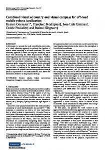
Training builds the map using input examples. It is a competitive process, also called vector quantization. A low-dimensional(typically two dimensional) map discretizess the input space of the training samples. The map seeks to preserve the topological properties of the input space. A structure of this map consists of components called nodes or neurons. Associated with each node is a weight vector of the same dimension as the input data vectors and a position in the map space. Nodes are connected by edges, resulting in a (2D) grid. 3.3.1 Building the map Our proposal operates in Scale Invariant Feature Vectors Space, SIFT space, instead of image space, in other words, our space has n=131 values(128 by SIFT’s descriptor vector and 3 by feature’s pose). A Kohonen map must be created and trained to represent the space of descriptors. When a new input arrives, the topological map determines the feature vector of the reference node that best matches the input vector. To make clear the method we explain the Kohonen algorithm which is splited in three main modules: 1. Competition process, consist in finding in our network a minimum Euclidian distance between de input vector X and de weight vector W, fig 2. If we use the index i(x) to identify the neuron which best matches, called winning node, with a input vector X, so applying the condition below we determine i(x):

I(x)=argmin||X-Wj||

Fig. 2 Minimum distances

Visual Odometry and mapping for underwater Autonomous Vehicles

2.

7

Cooperative process, comprise in a winning node change lateral distance of his neighbors. For that is basically used a Gaussian function, fig 3:

Fig. 3 Gaussian Function

3.

Adaptation process, this method is responsible for self-organization of a characteristics map. For that it`s necessary a modification of weights vector W in each neuron in relation of a input vector. To perform it is used eq. 7.

Wj(n+1)= Wj(n) +η(n)hj,i(x)(n)(x- Wj(n))

(7)

where η is learning rate and hj,i(x) is Gaussian decay function. The Growing Cell Structures method allows creation and removal of the nodes during the learning process. The Algorithm constrains the network topology to k-dimensional simplies where by K is some positive integer chosen in advance. In this work, the basic building block and also the initial configuration of each network is a K=2-dimensional simplex. For a given network configuration a number of adaptation steps are used to update the reference vectors of the nodes and to gather local error information at each node. This error information is used to decide where to insert new nodes. A new node is always inserted by splitting the longest edge emanating from the node q with maximum accumulated error. In doing this, additional edges are inserted such that the resulting structure consists exclusively of k-dimensional simplices again, see fig. 4.

Robot Localization and Map Building

8

Fig. 4 Illustration of cell insertion

To remove nodes, After a user-specified number of iterations, the cell with the greatest mean Euclidian distance between itself and its neighbors is deleted and any cells within the neighborhood that would be left “dangling” are also deleted, see fig. 5.

Fig. 5 Illustration of cell deletion: Cell A is deleted. Cells B and C are within the neighborhood of A and would be left dangling by removal of the five connections surrounding A, so B and C are also deleted.

After a set of training steps, the kohonen map represents the descriptors space. This SOM can be used to locate the robot during the navigation.

3.3.2 Location the robot on the map New frames are captured during the navigation. For each new frame F, SIFT calculates a set of m keypoints Xi, see equation 6. A n=131 dimensional descriptor vector is associated to each keypoint. We use the trained SOM to map/locate the robot in the environment. A mapping stage is runned m times. For each step i there will be one single winning neuron, Ni: the neuron whose weight vector lies closest to the input descriptor vector, Xi. This can be simply determined by calculating the Euclidean distance between input vector and weight vectors. After the m steps we have a set of m winner nodes, Ni, associated with each one feature descriptor, Xi. With the pose information of m pairs (Xi, Ni), we can use the homography concept to obtain a linear matrix transformation, H SOM. Equation 8 gives the map localization of center of the frame, XC’= (xc’, yc’):

Xc’=HSOM * XC,

Visual Odometry and mapping for underwater Autonomous Vehicles

9

Where XC is the position of the center of the frame. Moreover the final topological map allows the navigation in two ways: through target positions or visual goals. From the current position, graph search algorithms like Dijkstra [Dijkstra59] or A* algorithm [Dechter85] can be used to search a path to the goal.

4. System Implementation, Tests and Results In this work, it was developed the robot presented in figure 6. This robot is equipped with a Tritech Typhoon Colour Underwater Video Camera with zoom, a miniking sonar and a set of sensors (altimeters and accelerometers) [Centeno07]. Due this robot is experimental phase, it is impossible to put it to work in the sea. The acquition of some reference to experiements is very hard in this kind of environment, too. Considering this situation, this work use a simulated underwater conditions proposed by [Arrredondo05]. Using it, different undersea features were applied in the images, like turbidity, sea snow, non-linear illumination, and others, simulating different underwater conditions. Table I shows the apllied features (filters).

Figure 6. ROVFURGII in test field

Robot Localization and Map Building

10

TABLE I UNDERSEA FEATURES FOR EACH DISTORTION USING IN THE TESTS. Distortion Light Source distance (m) Attenuation value % Gaussian noise  Gray level minimum Number of flakes of sea snow

1 0.2 0.05 2 20 30

2 0.22 0.05 2 30 30

3 0.25 0.06 2 20 30

4 0.25 0.05 4 20 30

5 0.3 0.05 4 20 30

The visual system was tested in a desktop Intel Core 2 Quad Q6600 computer with 2 Gb of DDR2-667 RAM. The camera is NTSC standard using 320x240 pixels at a maximum rate of 29.97 frames per second.

4.1 The method in different underwater features The visual system was tested in five different underwater environments, corresponding the image without distortion and first four filters presented in table I(the effects were artificially added to the image). Figure 7 enumerates the detected and matching keypoints obtained in a sequence of visual navigation. Even though the number of keypoints and correlations has diminished with the quality loss because of underwater conditions, is still possible to localize the robot, according figure 8. In this figure, the motion referencial is represented in blue(legended as “Odometry”), executed by a robotic arm composed by an Harmonic Drive PSA-80 actuator with a couple encoder supplying angular readings in each 0.651 ms, with a camera coupled to this. It allows the reference system a good precision, 50 pulses per revolution. Therewith, it is possible to see that our approach is robust to underwater environment changes. All graphics in this chapter use centimeter as metric unit, including figure 8.

Visual Odometry and mapping for underwater Autonomous Vehicles

11

Fig. 7. Number of keypoints detected and true correlation during the robotic arm movement.

12

Robot Localization and Map Building

Fig. 8. Position determinated by the robotic arm odometry and a visual system, without and with distortion.

4.2. Online Robotic Localization Tests were performed to evaluate the SIFT algorithm performance considering a comparison with another algorithm for robotic localization in underwater environment: KLT [Plakas00][Tommasini98][Tomasi91][Shi94].

Visual Odometry and mapping for underwater Autonomous Vehicles

13

Figure 9 shows the performance results using and KLT methods. SIFT has obtained an average rate of 4.4 fps over original images, without distortion, and a rate of 10.5 fps with the use of filter 5, the worst distortion applied. KLT presented higher averages, 13.2 fps and 13.08 fps, respectively. Note that SIFT has worst performance in high quality images because the large amount of detected points and, consequently, because the higher number of descriptors to be processed. The KLT, instead, keeps an almost constant performance. However, due to he slow dynamic associated with undersea vehicle motion, both methods can be applied to online AUV SLAM. The green cross represent the real final position and the metric unit is centimeter. The SIFT results related to the robot localization were considered satisfactory, even with extreme environment distortions (filter 5). In the other hand, KLT gives insatisfying results for both cases, onde it is too much susceptible to the robot`s depth variation, or image scale, that occurs constantly in the AUV motion despite the depth control. 4.3. Robustness to Scale A set of tests were performed to estimate the robustness of the proposed system to the sudden scale variantion. In this case, a translation motion with height variation was performed with the camera to simulate a deeper movement of the robot in critical conditions. The figure 10 shows the SIFT results, considered satisfactory, even in critical water conditions. Considering the use of some filters in extreme conditions, SIFT is superior to KLT although it shows an inexistent movement in Y axis. Over the tests, SIFT has shown an average rate of 6.22 fps over original images captured by the camera and a rate of 7.31 fps using filter 1 and 10.24 fps using filter 5. The KLT have shown 12.5, 10.2 and 11.84 fps, respectively. The green cross represent the real final position, is the same for all graphics in figure 10, the metric is centimeter.

14

Robot Localization and Map Building

Fig. 9. Real Robot Localization in online system, without and with artificial distortion.

Visual Odometry and mapping for underwater Autonomous Vehicles

Fig. 10. Localization with translation and scale movement without and with distortion.

15

16

Robot Localization and Map Building

4.4. Topological Maps Tests to validate the mapping system proposed were performed. For example, during a navigation task s set of 1026 frames were captured. From these frames, a total of 40.903 vectors are extracted from SIFT feature algorithm. To build the map, 1026 frames and 40903 keypoints are presented to the SOM. Figure 11 show the final 2D map, discretizing the input space of the training samples.

Fig. 11. Topological Map generated by ROVFURGII in movement.

Visual Odometry and mapping for underwater Autonomous Vehicles

a)

17

Building the map: when a new keypoint arrives, the topological map determines the feature vector of the reference node that best matches the input vector. The Growing Cell Structures (GCS) method allows the creation and removal of the nodes during the learning process. Table II shows intermediate GCS adaptation steps with number of frames, keypoints and SOM nodes. After the training stage (1026 frames), the kohonen map represents the relevant and noise tolerant descriptors space using a reduced number of nodes. This SOM can be used to locate the robot during the navigation. TABLE II BUILDING THE MAP WITH GCS ALGORITHM

Frames 324 684 1026

b)

Keypoints 20353 35813 44903

Nodes 280 345 443

Location of robot on the map: New frames are captured during the navigation. We use the trained SOM to map/locate the robot in the environment. Figure 12 shows the estimated position of a navigation task. In this task the robot crosses three times the position 0.0. In this figure we can see the position estimated by both the SOM map (blue) and only by visual odometry (red). In the crossings, table III shows the normalized errors of positioning in each of the methods. The reduced error associated with the SOM localization validate the robusteness of topological approach.

TABLE III NORMALIZED LOCALIZATION ERRORS OF ONLY VISUAL ODOMETRY AND SOM. Visual Odometry SOM 0.33 0.09 0.68 0.35 1.00 0.17

Robot Localization and Map Building

18

Fig. 12. Distance Y generated by ROVFURGII in movement.

5. Conclusion This work proposed a new approach to visual odometry and mapping of a underwater robot using only online visual information. This system can be used either in autonomous inspection tasks or in control assistance of robot closed-loop, in case of a human remote operator. A set of tests were performed under different underwater conditions. The effectiveness of our proposal was evaluated inside a set of real scenario, with different levels of turbidity, snow marine, non-uniform illumination and noise, among others conditions. The results have shown the SIFT advantages in relation to others methods, as KLT, in reason of its invariance to illumination conditions and perspective transformations. The estimated localization is robust, comparing with the vehicle real pose. Considering time performance, our proposal can be used to online AUV SLAM, even in very extreme sea conditions. The correlations of interest points provided by SIFT were satisfying, even though with the presence of many outliers, i.e., false correlations. The proposal of use of fundamental matrix estimated in robust ways in order to remove outliers through RANSAC and LMedS algorithms. The original iintegration of SIFT and topological maps with GCS for AUV navigation is a promising field. The topological mapping based on Kohonen Nets and GCS showed potencial potential to underwater SLAM applications using visual information due to its robustness to sensory impreciseness and low computational cost. The GCS stabilizes in a limited number of nodes sufficient to represent a large number if descriptors in a long sequence of frames. The SOM localization shows good results, validating its use with visual odometry.

Visual Odometry and mapping for underwater Autonomous Vehicles

19

6. References [Arredondo05] Miguel Arredondo and Katia Lebart. A methodology for the systematic assessment of underwater video processing algorithms. Oceans - Europe, 1:362–367, June 2005. [Bay06] H. Bay, T. Tuytelaars, and L.booktitle = SURF: Speeded Up Robust Features Van Gool. Surf: Speeded up robust features. In 9th European Conference on Computer Vision, pages 404–417, 2006. [Booij07] O. Booij, B. Terwijn, Z. Zivkovic, and B. Krose. Navigation using an appearance based topological map. In IEEE International Conference on Robotics and Automation, pages 3927–3932, April 2007. [Centeno07] Mario Centeno. Rovfurg-ii: Projeto e construção de um veículo subaquático não tripulado de baixo custo. Master’s thesis, Engenharia Oceânica - FURG, 2007. [Dechter85] Rina Dechter and Judea Pearl. Generalized best-first search strategies and the optimality af a*. Journal of the Association for Computing Machinery, 32(3):505–536, July 1985. [Dijkstra59] Edsger W. Dijkstra. A note on two problems in connexion with graphs. Numerische Mathematik, 1:269–271, 1959. [Fischler81] Martin Fischler and Robert Bolles. Random sample consensus: a paradigm for model fitting with applications to image analysis and automated cartography. Communications of the ACM, 24(6):381–395, 1981. [Fleischer00] Stephen D. Fleischer. Bounded-Error Vision-Based Navigation of Autonomous Underwater Vehicles. PhD thesis, Stanford University, 2000. [Fritzke93] Bernd Fritzke. Growing cell structures - a self-organizing network for unsupervised and supervised learning. Technical report, University of California - Berkeley, International Computer Science Institute, May 1993. [Garcia01] Rafael Garcia, Xavier Cufi, and Marc Carreras. Estimating the motion of an underwater robot from a monocular image sequence. In IEEE/RSJ International Conference on Intelligent Robots and Systems, volume 3, pages 1682–1687, 2001. [Garcia05] Rafael Garcia, V. Lla, and F. Charot. Vlsi architecture for an underwater robot vision system. In IEEE Oceans Conference, volume 1, pages 674–679, 2005. [Gracias02] N. Gracias, S. Van der Zwaan, A. Bernardino, and J. Santos-Vitor. Results on underwater mosaic-based navigation. In IEEE Oceans Conference, volume 3, pages 1588– 1594, october 2002. [Gracias00] Nuno Gracias and Jose Santos-Victor. Underwater video mosaics as visual navigation maps. Computer Vision and Image Understanding, 79(1):66–91, July 2000. [Hartley04] Richard Hartley and Andrew Zisserman. Multiple View Geometry in Computer Vision. Cambridge University Press, 2004. [Kohonen01] Teuvo Kohonen. Self-Organizing Maps. Springer-Verlag New York, Inc., Secaucus, NJ, USA, 2001.

20

Robot Localization and Map Building

[Lowe04] David Lowe. Distinctive image features from scale-invariant keypoints. International Journal of Computer Vision, 60(2):91–110, 2004. [Mahon04] I. Mahon and S. Williams. Slam using natural features in an underwater environment. In Control, Automation, Robotics and Vision Conference, volume 3, pages 2076–2081, December 2004. [Nicosevici07] T Nicosevici, R. García, S. Negahdaripour, M. Kudzinava, and J Ferrer. Identification of suitable interest points using geometric and photometric cues in motion video for efficient 3-d environmental modeling. In International Conference in Robotic and Automation, pages 4969–4974, 2007. [Plakas00] K. Plakas and E. Trucco. Developing a real-time, robust, video tracker. In MTS/IEEE OCEANS Conference and Exhibition, volume 2, pages 1345–1352, 2000. [Rousseeuw84] Peter Rousseeuw. Least median of squares regression. Journal of the American Statistics Association, 79(388):871–880, December 1984. [Se02] Stephen Se, David Lowe, and James Little. Mobile robot localization and mapping with uncertainty using scale-invariant visual landmarks. The International Journal of Robotics Research, 21(8):735–758, 2002. [Se05] Stephen Se, David Lowe, and James Little. Vision-based global localization and mapping for mobile robots. IEEE Transactions on Robotics, 21(3):364–375, June 2005. [Shi94] Jianbo Shi and Carlo Tomasi. Good features to track. In IEEE Conference on Computer Vision and Pattern Recognition, pages 593–600, 1994. [Tomasi91] Carlos Tomasi and Takeo Kanade. Detection and tracking of point features. Technical report, Carnegie Mellon University, April 1991. [Tommasini98] T. Tommasini, A. Fusiello, V. Roberto, and E. Trucco. Robust feature tracking in underwater video sequences. In IEEE OCEANS Conference and Exhibition, volume 1, pages 46–50, 1998. [Torr97] P. H. S. Torr and D. W. Murray. The development and comparison of robust methods for estimating the fundamental matrix. International Journal of Computer Vision, 24(3):271 – 300, 1997. [Xu97] Xun Xu and Shahriar Negahdaripour. Vision-based motion sensing for underwater navigation and mosaicing of ocean floor images. In MTS/IEEE OCEANS Conference and Exhibition, volume 2, pages 1412–1417, October 1997.