Jon Sporring and Christos Colios. Abstract. Structure in digitized images resides within two scales, the inner and outer scale. The inner scale is defined by the ...
FORTH-ICS / TR-259
September 1999
Uncommitted Size-Estimation of Image Structure Jon Sporring and Christos Colios
Abstract Structure in digitized images resides within two scales, the inner and outer scale. The inner scale is de ned by the sampling resolution, and the outer scale is given by the image size. However, some images contain almost no ne scale structure, and these may be down-sampled without essential loss of image detail. Likewise some images may be reduced in size by removing borders with no structure. Hence we de ne essential inner and outer scales. Such considerations are the essence of local size estimation: A textured patch in an image has an essential inner scale related to the structure of the primitive textons, and an essential outer scale given by the size of the patch. In this paper, several functionals are examined that automatically nd both the essential inner and outer scales in local neighborhoods of an image. In this preliminary work we present a general formulation for local scale selection, that is shown to be a generalization of Lindeberg's Blob-detector and its morphological equivalent, and we present promising results using locally orderless images.
Keywords: Linear Scale-Space, Gaussian Windows, Lyaponov Functionals,
Blob-Detection, Pseudo-Linear Scale-Spaces, Locally Orderless Images, Soft Histograms.
Uncommitted Size-Estimation of Image Structure� Jon Sporring and Christos Colios Institute of Computer Science, Foundation for Research and Technology { Hellas, Vassilika Vouton, P.O. Box 1385, GR-71110 Heraklion, Crete, Greece
Technical Report FORTH-ICS / TR-259 | September 1999
c Copyright 1999 by FORTH
Abstract Structure in digitized images resides within two scales, the inner and outer scale. The inner scale is de ned by the sampling resolution, and the outer scale is given by the image size. However, some images contain almost no ne scale structure, and these may be downsampled without essential loss of image detail. Likewise some images may be reduced in size by removing borders with no structure. Hence we de ne essential inner and outer scales. Such considerations are the essence of local size estimation: A textured patch in an image has an essential inner scale related to the structure of the primitive textons, and an essential outer scale given by the size of the patch. In this paper, several functionals are examined that automatically nd both the essential inner and outer scales in local neighborhoods of an image. In this preliminary work we present a general formulation for local scale selection, that is shown to be a generalization of Lindeberg's Blob-detector and its morphological equivalent, and we present promising results using locally orderless images.
Keywords: Linear Scale-Space, Gaussian Windows, Lyaponov Functionals, Blob-Detection,
Pseudo-Linear Scale-Spaces, Locally Orderless Images, Soft Histograms.
This work was supported by EC Contract No. ERBFMRY-CT96-0049 (VIRGO http://www.ics.forth.gr/virgo) under the TMR Programme. �
1 Uncommitted Size-Estimates Objects or textons in most images have no prede ned size, shape, or position, and a general tool for size-estimation should naturally be unbiased. While it is computational intractable to consider all object shapes, it is possible to choose a least committed shape, and examine all sizes and positions of this. As demonstrated in [1, 2], the dominating size of global textured images can be estimated with Lyaponov functionals and the Linear scale-space. The Linear scale-space is an uncommitted scale-space, that treats all positions, directions, and scales identically (see [3] and references therein for the history of Linear scale-space). Scale-spaces extend an image I with a scale parameter t such that image structure is simpli ed when t increases. The Linear scale-space is the solution to the Heat Di�usion equation @t L = �L (with @ as the di�erentiation operator and � as the Laplacian operator, i.e. @xx in the one dimensional case treated in this paper). The Green's function of the Heat Di�usion equation is the Gaussian kernel implying that the Linear scale-space is equivalent to convolving or smoothing an image I as, L(x; t) = G(x; t) � I (x) =
where G is the Gaussian kernel,
Z
G(x ? x0 ; t)I (x0 ) dx0 ;
1 exp ? jxj2 G(x; t) = (4�t)D=2 4t
(1)
!
q
of standard deviation � = t=2, and where D is the dimension of the image domain . With respect to the amount of structure, smoothing an image with a Gaussian kernel of standard deviation � is similar to downsampling by replacing each non-overlapping 2� � 2� neighborhood with its mean, as is typically done in the image pyramid [4]. However, in contrast to downsampling, Linear scale-space is analytical [5, theorem 20, p. 125]. For increasing t, it was observed in [1] that the image changes fastest, when the standard deviation of the Gaussian kernel is close to the smallest radius of dominating image structure. To give an intuitive explanation of this, consider a line of width 2r. Smoothing the line with a Gaussian of standard deviation � � r will have little e�ect on the appearance of the line, and a small increase in t will only cause a small, further deterioration of the line. I.e. the rate of the change in appearance is low. Conversely, smoothing with a Gaussian of standard deviation � � r will fully remove the line, and the rate of deterioration is again low. For symmetry reasons it is therefore concluded that the largest rate of change is when � � r. In the context of scale-spaces, the Lyaponov functionals [6] are particular interesting, since they are all monotonically increasing with scale and may thus serve as a measure of causality. A Lyaponov functional is de ned as, S (t) =
X �
x2
�
� L(x; t) ;
(2)
where � is a convex function, i.e. @vv �(v) > 0. Lyaponov functionals are invariant under permutation of space, and are therefore solely a function of the image values and their 2
frequencies (the gray-value histogram). The R�enyi and Tsallis entropies, the gray-value moments, and the multifractal spectrum are some one-parameter subclasses of the Lyaponov functionals that constitute complete subclasses: each has a one-to-one relation with the gray value histogram. It is thus natural to consider one such subclass, measure the amount of structure by S (t) and the rate of deterioration by � X � @S (t) = t �t L(x; t) @t L(x; t); c(t) = @ log t x2
(3)
where log t is the natural scale-parameter [7, 8, 9] in which change in structure is approximately linear. Although it seems to be a very hard problem to give analytical relations between the maxima of c and the size of even simple image structure, it has been demonstrated empirically that simple relations exist [1, 2].
2 Local Size-Estimates Typical images are not of single objects or single textures, but contain objects of various sizes and textures of various extends. It is therefore the aim of the following to develop an uncommitted method for local size-estimation. For local size-estimates, the introduction of a window function is unavoidable. Most images have no prede ned optimal window sizes, and local size-estimates must therefore consider all window sizes. In that view, it is not advisable to use anything but Gaussian (soft) windows, since these uniquely guarantee not to introduce spurious detail, when changing the window size [10]. Like the letter t is used to denote the scale of the image, the letter w will be used to denote the size of the window. In terms of structure, may t be considered as the local inner scale, while w is the local outer scale, and the ration w=t accounts for the degrees of freedom inside each window. In contrast to global Lyaponov functionals (2), local Lyaponov functionals, S (x0 ; t; w) =
X x2
�
G(x ? x0 ; w)� L(x; t)
�
(4)
will not be monotonic with scale, since structure may move inside the window when t is increased. However, the sum of local Lyaponov functionals is monotonically increasing with t: Lemma 1 For S given as (4) and @vv �(v) > 0, Px02 S (x0; t; w) is monotonically increasing with t. To prove this, remember that�the Gaussian is symmetric, implying that (4) may be written � �� as S (x0; t; w) = G(x; w) � � L(x; t) (x0 ). Since the mean value of any image is invariant under Gaussian convolution, the following equivalence holds: X x0 2
S (x0 ; t; w) =
3
X �
x2
�
� L(x; t) :
(5)
100
100
100
100
90
90
90
90
80
80
80
80
70
70
70
70
60
60
60
60
50
50
50
50
40
40
40
30
20
40
60
80
100
120
30
20
40
60
80
100
30
120
40
20
40
60
80
100
120
30
20
40
60
80
100
120
Figure 1: The Test Functions: The frequency and amplitude of right section is varied. Since the right-hand side of (5) is monotonically increasing with t [6, Theorem 5] so must the left-hand side. This completes the proof. The structure of S (x0; t; w) with respect to the window size is given by the Heat Di�usion equation, @w S = �S , for any �. In spite of Lemma 1, it does not seem to be any immediate advantage of restricting S to be a local Lyaponov functional, and the following study will be general. The global size-estimation is generalized by considering both the extrema of the gradient magnitude: v u u c(x; t; w) = t
! ! @S (x; t; w) 2 @S (x; t; w) 2 + @ log w : @ log t
For almost all images we will get at least one solution for every x. In general there is no guarantee that a solution exists, and there might well be more than one. To give an example, consider a ock of birds. At each point in the ock there is more than one scale of interest, e.g. the birds are at a low scale, and the ock at a considerable higher scale. In the experiments reported below we examine all solutions. Except for the most simple candidate for S , it has not been possible to perform a satisfying analytical analysis. Therefore, a simple family of one dimensional functions shown in Figure 1 have been designed to illustrate key properties of the candidates. These functions are called the Test Functions and consist of two areas with di�erent mean, periodically extended on a circle. The right plateau is twice the width of the left. Each plateau is a sinus function of various frequency and amplitude. In the top row, only the frequency of the sinus function is increased, and in the bottom row only the amplitude is increased. The sinus function of the small plateau is the same for all functions.
2.1 Maximizing the sum yields maximum of Laplacian
Possibly the simplest functional we can consider is, X S (x0 ; t; w) = G(x ? x0 ; w)L(x; t) x2
(6)
Since the Gaussian is symmetric, and smoothing is a semi-group in scale, the sum may be written as a single smoothing, Ssum (x; t; w) = G(x; t + w) � I (x) = G(x; t0 ) � I (x); 4
15
15
15
15
10
10
10
10
5
5
5
5
0
0
0
0
−5
−5
−5
−5
−10
−10
−10
−10
−15
−15
−15
−15
−20
−20
−20
20
40
60
80
100
120
20
40
60
80
100
120
20
40
60
80
100
120
−20
60
60
60
60
50
50
50
50
40
40
40
40
30
30
30
30
20
20
20
20
10
10
10
10
20
40
60
80
100
120
20
40
60
80
100
120
20
40
60
80
100
120
20
20
40
40
60
80
100
120
60
80
100
120
Figure 2: Top row shows the values of csum(x0; t0 ) at the extremal points along log t0 for each point x0 forqeach of the Test Functions in Figure 1. Bottom row shows the corresponding kernel sizes t0=2. showing that the system only has one independent smoothing parameter t0 . Using the Heat Di�usion equation the function c may be written as, @Ssum = t�Ssum; @ log t0
csum (x; t0 ) =
resulting in Lindeberg's Blob-detector [11, pp. 325{328]. As an example, consider the function, f (x; v ) = a cos(2�vx): Smoothing f with a Gaussian kernel of standard deviation � yields, f (x; v; t) = exp
�
�
?(2�v)2t a cos(2�vx):
In order to nd the scale of maximum change of f by log t we have to nd the zero-crossing of the second derivative with respect to log t, @f 2 @ 2 f @ 2 f (x; v; t) = t + t @t2 = 0: @ (log t)2 @t
The solution is readily found to be,
2 ; (2�v)2 independently on the amplitude a for almost all x. For more complicated functions the results are not quite as simple. In Figure 2 the maximum values of csum and corresponding scales t0 are shown for each point in each of the Test Functions. As can be seen from these gures, most points x have several solutions. t=
5
Examining the bottom row, we observe that there are two re-occurring families of solutions topping at (x = 21; �0 ' 15) and (x = 85; �0 ' 28), which correspond to the width of the small and large plateau of the Test Figures. Corresponding families may be found in the top row. Further, we see that a secondary set of solutions occur at (�0 ' 6). For the Test Figures with high frequencies at the low plateau, these solutions are periodic with a period identical to the Test Functions. Such behavior is typical: The plateaus de ne large scale structure, while the sinusoids de ne a small scale structure. Each can be found using csum.
2.2 Weighted Monotonic Functions yields Pseudo-Linear ScaleSpaces
The function Ssum does not distinguish between the inner and outer scale. A simple extension is to introduce a monotonic function �, @v �(v) > 0, as follows: Spseudo (x; t; w; �) =
=
�X � ? 1 � G(y ? x; w)�(L(y; t)) y2
� � �?1 G(x; w) � �(L(y; t)) :
This is a Pseudo-linear scale-space on L evolving according to @w L = �L + �(L)jjrLjj2 [12], where �(v) = @@vvv �(�(vv)) is the nonlinearity parameter. The Pseudo-linear scale-space will be identical to the Linear scale-space on L, when �(v) = 0. However, when � ! �1, the Pseudo-linear scale-space will converge to the morphological dilation or erosion scale-spaces on L (with the quadratic structuring element �jjxjj2=(4w)). Other functions �(v) would lead to a non-linear mixing of the two. Consider the example of weighted gray-value moments of L, i.e. �moment(v) = v�. For a particular �, the non-linearity parameter will be �moment(v) = (� ? 1)=v. Further, �moment(v ) ! 0 when � ! 1, and �moment(v ) ! �1 when � ! �1. Hence Gaussian weighted gray-value moments of L is an example of a Pseudo-linear scale-space. For xed w = 0, both cdilation and cerosion will behave as (2.1). Conversely, in Figures 3 and 4 the selected window-size is shown, based on cdilation and cerosion for xed value t = 0. The dilation process will evolve a function towards its global maximum, hence, the function cdilation is high on the low plateau and low on the high plateau. Conversely, the function jcerosionj is high on the high plateau and low on the low plateau. Further, the selected window sizes peak at the middle of the low and high plateau for the respective morphological processes. The selected window size is largest for the low plateau at the peak corresponding to the di�erence in the size of the two plateaus. Finally, the ne structure relating to local extrema inside each plateau can be interpreted in the same manner. Simultaneous scale-selection of both t and w seem to be dominated by the one-dimensional cases, where either t = 0 or w = 0, as explained above. In Figure 5 examples of cdilation and cerosion are shown, as a function of scale and window size for a selected number of spatial positions of a single Test Function. The two processes are close to being symmetric with respect to the center of the plateaus. In the center of the high plateau (x = 21), cdilation is basically independent on w making the selection of w highly uncertain. Similarly, the selection of t is highly uncertain at the center of the low plateau (x = 85) for cdilation. We, 6
9
9
9
9
8
8
8
8
7
7
7
7
6
6
6
6
5
5
5
5
4
4
4
4
3
3
3
3
2
2
2
2
1
1
1
0
20
40
60
80
100
120
0
20
40
60
80
100
0
120
1 20
40
60
80
100
120
0
60
60
60
60
50
50
50
50
40
40
40
40
30
30
30
30
20
20
20
20
10
10
10
10
20
40
60
80
100
120
20
40
60
80
100
120
20
40
60
80
100
120
20
20
40
40
60
80
100
120
60
80
100
120
Figure 3: Top row shows the values of cdilation(x0; t0 ) at the extremal points along log w for xed t = 0 and each point x0 of the Test Functions in Figure 1. Bottom row shows the p corresponding kernel sizes w. therefore, conclude that at the limit of � = �1, simultaneous selection of t and w does not seem practical.
2.3 Soft Histograms
The soft histograms de ned by Koenderink and van Doorn [10] make the study of local histograms well-posed. To accomplish this 3 parameters are introduced: t, , and w. The parameter t allows a smooth analysis of the pixel resolution between the inner and outer scale, parameter smoothly varies the resolution of the image intensities between a single intensity and the number of intensities in the original image, and nally parameter w controls the size of the soft window function at a given position. To calculate the soft histogram, the image I is rst smoothed to obtain L(x; t) as (1). In regions of an image where the intensity is close to constant, the location of isophotes are typically erratic. As suggested by Gri�n [13], a �well-posed,2 �soft de nition of intensities is obtained when the isophote i is replaced with exp ? (L(x2;t )2?i) . In this manner, an isophote will be spread out over almost constant regions in an image, where controls the amount of spreading. Finally, local histograms are obtained by weighing each soft isophote with a Gaussian window of width w, and we obtain ! Z ( L(x; t) ? i)2 H (i; x0 ; t; ; w) = G(x; x0 ; w) exp ? dx; (7) 2 2
where the function H gives the frequency of the soft intensity i in the point x0 . For our purpose we de ne Shistogram as, X Shistogram = ? P (i; x0 ; t; ; w) log P (i; x0 ; t; ; w); i
7
0
0
0
0
−1
−1
−1
−1
−2
−2
−2
−2
−3
−3
−3
−3
−4
−4
−4
−4
−5
−5
−5
−5
−6
−6
−6
−6
−7
−7
−7
−7
−8
−8
−8
−9
20
40
60
80
100
−9
120
20
40
60
80
100
−8
−9
120
20
40
60
80
100
120
−9
60
60
60
60
50
50
50
50
40
40
40
40
30
30
30
30
20
20
20
20
10
10
10
10
20
40
60
80
100
120
20
40
60
80
100
120
20
40
60
80
100
120
20
40
60
80
100
120
20
40
60
80
100
120
Figure 4: Top row shows the values of cerosion(x0 ; t0) at the extremal points along log w for xed t = 0 and each point x0 of the Test Functions in Figure 1. Bottom row shows the p corresponding kernel sizes w.
100 90 80
21
70 60 50 40 30
20
40
60
80
100
dilation
85
2
2
2
4
4
4
6
6
6
8
8
8
10
10
10
12
12
12
14
14
14
16
16 5
erosion
42
120
10
16
15
5
10
15
2
2
2
4
4
4
6
6
6
8
8
8
10
10
10
12
12
12
14
14
14
16
16 5
10
5
10
15
5
10
15
16
15
5
10
15
Figure 5: The functions cdilation and cerosion as a function of scale and window size for a selected number of spatial positions of the rightmost Test Function in Figure 1. 8
0.07
0.07
0.07
0.07
0.06
0.06
0.06
0.06
0.05
0.05
0.05
0.05
0.04
0.04
0.04
0.04
0.03
0.03
0.03
0.03
0.02
0.02
0.02
0.02
0.01
0.01
0.01
0.01
0
0
0
20
40
60
80
100
120
20
40
60
80
100
120
20
40
60
80
100
0
120
60
60
60
60
50
50
50
50
40
40
40
40
30
30
30
30
20
20
20
20
10
10
10
10
20
40
60
80
100
120
20
40
60
80
100
120
20
40
60
80
100
120
60
60
60
60
50
50
50
50
40
40
40
40
30
30
30
30
20
20
20
20
10
10
10
10
20
40
60
80
100
120
20
40
60
80
100
120
20
40
60
80
100
120
20
40
60
80
100
120
20
40
60
80
100
120
20
40
60
80
100
120
Figure 6: Top row shows the maximum value of chistogram, where both are maximum for each point of the Test Functions in Figure 1, and middle and bottom rows shows the corresponding t and w scales. where P is the normalized soft histogram, H (i; x0 ; t; ; w) P (i; x0 ; t; ; w) = P : j H (j ; x0 ; t; ; w )
In Figure 6 the simultaneous selection of scale and window-size is shown. The function chistogram peaks at the center of the two plateaus and at the edges. Likewise, both t and w peak at the center of the plateaus, but the selected w's near the edges seem erratic. It is further observed that at the center of the plateaus, the selected t's and w's are very similar for all Test Functions, implying that the ne structure is ignored. Finally, the peaks in w at x = 21 and x = 85 are proportional to the size of the corresponding plateaus.
3 Summary Scale-selection is in essence a local process. In this preliminary work local scale-selection is cast in the avor of local Lyaponov functionals. Certainly, local Lyaponov functionals cannot be monotonic since information is allowed to move across window borders. While it can easily be shown that the sum of all local Lyaponov functionals is monotonic, this property does not immediately suggest an application. Therefore, this paper focused on a larger 9
class of functionals, and this formulation is shown to be a generalization of some already known scale-selection mechanisms: The Blob-Detector and its morphological equivalent. For simultaneous detection of both window size and smoothing it seems that the concept of locally orderless images is the most powerful.
References [1] Jon Sporring and Joachim Weickert. Information measures in scale-spaces. IEEE Trans. on Information Theory, 45(3):1051{1058, 1999. Special Issue on Multiscale Statistical Signal Analysis and Its Applications. [2] Masaru Tanaka, Takashi Watanabe, and Taketoshi Mishima. Tsallis entropy in scalespaces. In L. J. Latecki, R. A. Melter, D. M. Mount, and A. Y. Wu, editors, SPIE conference on Vision Geometry VIII, volume 3811 of Proceedings of SPIE, October 1999. [3] J. Weickert, S. Ishikawa, and A. Imiya. On the history of Gaussian scale-space axiomatics. In Jon Sporring, Mads Nielsen, Luc Florack, and Peter Johansen, editors, Gaussian Scale-Space Theory, chapter 4, pages 45{59. Kluwer Academic Publishers, Dordrecht, The Netherlands, 1997. [4] Peter J. Burt and Edward H. Adelson. The Laplacian pyramid as a compact image code. IEEE Transactions on Communications, COM-31(4):532{540, 1983. [5] David Colton. Partial Di�erential Equations. Random House, New York, 1988. [6] J. Weickert. Anisotropic di�usion in image processing. Teubner Verlag, Stuttgart, 1998. [7] J. J. Koenderink. The structure of images. Biological Cybernetics, 50:363{370, 1984. [8] L. Florack. Image Structure. Computational Imaging and Vision. Kluwer Academic Publishers, Dordrecht, 1997. [9] Jon Sporring and Joachim Weickert. On generalized entropies and scale-space. In ScaleSpace Theory in Computer Vision, Proc. 1st International Conference, volume 1252 of Lecture Notes in Computer Science, pages 53{64, Utrecht, The Netherlands, July 1997. [10] Jan J. Koenderink and Andrea J. van Doorn. The structure of locally orderless images. International Journal of Computer Vision, 31(2/3):159{168, 1999. [11] T. Lindeberg. Scale-Space Theory in Computer Vision. The Kluwer International Series in Engineering and Computer Science. Kluwer Academic Publishers, Boston, USA, 1994. [12] Luc Florack, Robert Maas, and Wiro Niessen. Pseudo-linear scale-space theory. International Journal of Computer Vision, 31(2/3):247{259, 1999. [13] L. D. Gri�n. Scale-imprecision space. Image and Vision Computing, 15:369{398, 1997. 10