Understanding and Solving Flip-Ambiguity in Network ... - IEEE Xplore

Understanding and Solving Flip-Ambiguity in Network Localization via Semidefinite Programming Stefano Severi† , Giuseppe Abreu , Giuseppe Destino and Davide Dardari†

†

Dipartimento di Elettronica Informatica e Sistemistica, Universit`a degli Studi di Bologna Via Venezia 52, Cesena, Italy 47023 Email: {stefano.severi,ddardari}@ieee.org  Centre for Wireless Communications, University of Oulu, Finland P.O.Box 4500 FIN-90014 Email: {destino,giuseppe}@ee.oulu.fi Abstract—We employ the semidefine programming (SDP) framework to first analyze, and then solve, the problem of flipambiguity afflicting range-based network localization algorithms with incomplete ranging information. First, we study the occurrence of flip-ambiguous nodes and errors due to flip ambiguity by considering random network topologies with successively smaller connectivity ranges RMax > RMax − ΔR > · · · > RU > RL , and employing an SDP-based unique localizability test to detect the limiting connectivity ranges RU and RL that are respectively sufficient and un-sufficient to ensure unique localizability. Then, we utilize this information to construct an SDP formulation of the localization problem with Genie-aided constraints, which is shown to resolve flip-ambiguities. Finally, we derive a flipambiguity-robust network localization algorithm by relaxing the Genie-aided constraints onto feasible alternatives. Finally, the performance of the so-obtained localization algorithm is studied by Monte-Carlo simulations, which reveal a substantial improvement over the conventional SDP-based algorithm.

I. I NTRODUCTION Flip-ambiguity is one of the most significant potential problems faced by network localization algorithms. This problem arises when the connectivity available in the network is insufficient to ensure that no node to be localized admits multiple location estimates that are equally likely, as per the cost-function that defines the localization algorithm itself. The typical effect of such multiple and equivalent solutions is that optimization methods employed to find the location estimates are unable to distinguish amongst possibly very different topological configurations that yield equal cost-values, often resulting in catastrophic errors [1]. Due to its very nature, there is little hope to find a solution to such a problem through the development of new optimization methods. Arguably, this explains the predominant approach found in current related literature which is to identify and eliminate flip-ambiguous nodes from the set of targets to be localized [2], [3]. In other words, the currently common approach amounts to avoiding the flip-ambiguity problem and attempt to minimize the location error of the less problematic nodes at the expense of the ones that are harder to localize. While such an approach does improve the performance of localization algorithms – as measured by the errors over the nodes effectively localized – the underlying principle of simply leaving flip-ambiguous nodes without any location estimates may be unacceptable in many applications. In this article we make steps towards solving, rather than avoiding, the flip-ambiguity problem by developing a tech-

nique that produces location estimates for all nodes in the network while minimizing the harmful effect of flip-ambiguitiy. To this end, we start by employing the unique localizability test constructed out of a semidefine programming (SDP) formulation of the network localization problem [4] to study the statistical occurrence of flip-ambiguous nodes. The study reveals that in the majority of situations the number of flipambiguous nodes is much smaller than the total number of nodes to be localizable, suggesting that sufficient information remains in the connectivity of non-uniquely localizable networks to enable flip-ambiguous nodes to be localized as well. Instrumented by that insight, we proceed to study the relationship between unique localizability and constraints that can be imposed over unmeasured distances so as to enable a stable solution to be obtained from the SDP-based localization algorithm. This leads to an impractical (Genie-aided) SDP formulation of the network localization problem which is found indeed to be capable of localizing, with a small average error, all nodes out of network afflicted by flip-ambiguity. Finally, a concrete solution is obtained by relaxing the unfeasible conditions of the Genie-aided approach and combination with a refining post-processing [5]. An exhaustive Monte Carlo analysis of the performance obtained with the proposed method confirms its ability to resolve flip-ambiguity, at the expense of a negligible increase in localization error. II. L OCALIZABILITY T EST AND E DGE - BOUNDING Throughout the article we shall consider the localization problem for networks lying in the two-dimensional space (η = 2), which can be studied using the unique-localizability test provided in [4]. Here, a network is understood as a set of N interconnected nodes randomly deployed with uniform distribution inside a square of unitary1 length ( = 1). Nodes whose locations are know exactly and a priori will be referred to as anchors, while the remaining nodes will be called targets. We shall refer to the total number of nodes N of a network also as its size, and all networks studied will contain A = 3 anchor nodes, such that for any realization there are T = N − A target nodes. We adopt the scaled unitary disk graph (UDG) model, so that a pair of target nodes at locations (column vectors) xi and 1 This is without loss of generality and amounts to a normalization of all distance quantities.

978-1-4244-4148-8/09/$25.00 ©2009 This full text paper was peer reviewed at the direction of IEEE Communications Society subject matter experts for publication in the IEEE "GLOBECOM" 2009 proceedings.

xj , is said to be connected if and only iff (iff) their distance  dij  xi − xj  = xi − xj , xi − xj  ≤ R, where  ·  denotes the Euclidean norm, · denotes inner product, and R is a given connectivity range. Likewise, an anchor at the location ak is connected to a target located at xj iff dkj  ak − xj  ≤ R. It will be assumed that all dij ≤ R and dkj ≤ R are known. Since the location of all anchors and their mutual distances are known, anchors are, to all effect considered to be interconnected. For each network as described above there is an associated graph G([A; X], H), where A  [a1 , · · · , aA ] is the anchor node coordinate matrix carrying the column vectors with the location of all anchors, X  [x1 , · · · , xT ] is the target node coordinate matrix carrying the column vectors with the location of all targets, and H is the incidence matrix defined below.   HA HT 0 (1) H[N × N ·(N −1) ]  0 EA ET 2

find X ∈ Rη×T , Y ∈ RT ×T such that eTij Yeij = d2ij ,  a  k 2 T T Z ak ej e = dkj ,

(7)

j

Y = XT X, ∀k ≤ A; i, j ≤ T. The SDP variation of the network localization problem formulated above is obtained [4] by relaxing the equality constraint Y = XT X into the positive semidefinite condition Z  0. Under such relaxation and with elementary algebra introduced to eliminate the variables X and Y we arrive at maximize 0 subject to Z1:η,1:η = Iη tr(CT Z) = d2ij , tr(CA Z) =

A-by- A·(A−1) 2

In the above, HA and ET are the and T -byincidence matrices of the sub-graphs containing only anchor nodes, and only target nodes, respectively. In turn, HT is a block-diagonal matrix with the structure: ⎤ ⎡ b1 0 .. ⎦, HT  ⎣ (2) . 0 bA T ·(T −1) 2

Then, the network localization problem can then be stated as follows

(8)

d2kj ,

Z  0, where Z1:η,1:η is the η × η first-minor of Z and the constants CT and CA are defined as 

0[η×1]  (9) CT  0[1×η] eTij , eij   ak  T T CA  e (10) ak ej . j

where each 1-by-T block bk is a row vector whose j-th element bkj is 1 iff the k-th anchor is connected to the jth target. Finally, the matrix EA is formed by appended diagonal matrices such that

EA  D1 · · · DA ,

(3)

where the j-th element of each T -by-T diagonal matrix Dk is −1 iff the k-th anchor is connected to the j-th target. The target-to-target and anchor-to-target squared-norms (or squared-distances) can be concisely written as (4) xi − xj 2 = eTij XT Xeij = d2ij ,

   a Iη   k Iη X ak − xj 2 = aTk eTj = d2kj , (5) e T j X ∀k ≤ A; i, j ≤ T, where eij is the column vector of ET whose i-th and j-th elements are 1 and −1, respectively, while ej is the column vector of EA whose j-th element is −1. Define the matrix 

Iη X . (6) Z XT Y

We are now ready to invoke the unique localizability theorem by So and Ye [4]. Theorem 1 - Unique Network Localizability A network represented by the graph G([A; X], H) is unique localizable iff rank(Z) = η. Proof: See [4]. Corollary 1.1 - Identification of Non-localizable Nodes All flip-ambiguous nodes of a non-uniquely localizable network G([A; X], H) can be identified. Proof: Biswas and Ye [6] demonstrate that the trace of the difference matrix Y − XT X can be used as a measure of the quality of localization. The smaller the trace, the higher accuracy of the estimation. In particular, the j-th diagonal element of Y − XT X is proportional to the accuracy of the position estimation of the j-th target node.  Using Corollary 1.1 we are able to study the statistics of the number of flip-ambiguous nodes in randomly generated networks of different sizes. Notice that in the context under consideration, since all known distances dij and dkj are errorfree, the only reason for a node not to be localizable is due to flip-ambiguity. If the the j-th diagonal element of Y − XT X is greater than 0, the corresponding node is flip-ambiguous. To illustrate typical results obtained, histograms of α for various N are shown in in figure 1. We recall that in all cases considered the number of anchors is the minimum possible, i.e., A = 3.

978-1-4244-4148-8/09/$25.00 ©2009 This full text paper was peer reviewed at the direction of IEEE Communications Society subject matter experts for publication in the IEEE "GLOBECOM" 2009 proceedings.

As can be seen, the study shows that the number of flipambiguous target nodes that make a network non-uniquely localizable is, in the majority of cases, a small number, that is, α N . For example, for networks of sizes N = 10, it is found that α = 1 approximately 45% of the time and α ≤ 2 over 60% of the time. Likewise, for N = 25, α ≤ 3 also for approximately 60% of the times. In all cases, it is evident that the number of ambiguous nodes is typically only a small fraction of the total number of nodes in the network. This observation, which albeit empirical is solidly legitimized by the unique localizability test, suggests that the prevailing approach in the literature related to the flipambiguity problem in network localization [7], [8] may be too pessimistic. Indeed, current techniques aim to avoid, rather than solve, flip-ambiguity, by eliminating ambiguous targets from the topology over which localization is attempted. The approach is justified by the well-known fact that flipambiguity may lead to catastrophic localization errors, but has the drawback of leaving the remaining nodes without any location estimate, which may be unacceptable in many applications. The results obtained from Corollary 1.1, however, motivated us to investigate a technique to resolve flip-ambiguities, ultimately enabling the localization of all nodes in the network. The mathematical rational behind such a technique, which is latter presented in section IV, is described in the sequel. 50

45

45

40

40

35

35

Occurences (%)

30

25

20

20

15

15

10

10

5

5

0

1

2

α

3

4

5

6

0

7

2

4

(a) N = 10

α

8

10

12

45

40

40

35

35

Occurences (%)

30

30

25

25

20

20

15

15

10

10

5

5

2

4

6

8

α

10

12

14

16

0

Consider the network G([A; X], H) formed by such nodes under a connectivity range √ R. In the unitary square, a connectivity range RMax = 2 ensures that the network is fully connected and thus, uniquely localizable. For R < RMax , the unique localizability of G([A; X], H) clearly depends on the relationship between the connectivity range R and average pairwise distance d¯N , which for N = 10 and N = 25, for instance, are d¯10 ≈ 0.23 and d¯25 ≈ 0.15, respectively. We are interested in a pair of connectivity ranges RU and RL = RU − ΔR such that the network is uniquely localizable under RU and not under RL . In order to find the edge bounds RU and RL , consider the decreasing sequence RMax > RMax − ΔR > · · · > RU > RL , where ΔR RMax − d¯N . For the cases to be studied here (10 ≤ N ≤ 25), RMax − d¯N  1.2, so that it is enough to set ΔR = 0.05 in order to obtain sufficiently tight bounds. Let HU and HL be the incidence matrices corresponding to the uniquely localizable and the non-uniquely localizable networks obtained with RU and RL respectively. By comparing HU against HL , one is able to identify the set of distances d˜ij which, if not measured, results in the network not being uniquely localizable. Thus define  ˜T 0 0 H , ˜A E ˜T 0 E 

0[η×1]  ˜T  C ˜Tij , 0[1×η] e ˜ij e   ak  T T ˜ CA  e ˜j , ak e ˜ j

Occurences (%)

50

45

0

6

(b) N = 15

50

(12)

30

25

 d¯N = 0.512 2/N .

˜  HU − HL = H

Occurences (%)

50

Applying this result to the case where N nodes lye in the square, and using  = 1 yields

2

4

6

8

10

α

12

14

16

18

20

22

(c) N = 20 (d) N = 25 Fig. 1. Distribution of the number of flip-ambiguous target nodes α for networks of different sizes N = {10, 15, 20, 25}.

(13) (14) (15)

˜ T whose i-th and j-th ˜ij is the column vector of E where e ˜j is the column elements are 1 and −1, respectively, while e ˜ A whose j-th element is −1. vector of E Now the network G([A; X], HL ), despite failing the unique localizability test of Theorem 1, can be localized using the SDP formulation of the network localization given in (8), augmented by additional constraints. Specifically, maximize 0 subject to Z1:η,1:η = Iη tr(CT Z) = d2ij ,

III. L OCALIZATION WITH G ENIE - AIDED E DGE -B OUNDING Consider the randomly deployed set of nodes as described in section II. The median distance between two nodes lying in an -by- square was shown in [9] to be d¯2 = 0.512.

(11)

tr(CA Z) = d2kj , . . . . . . . .. . . . .  ........ 2 ˜ RL < tr CT Z ≤ RU2 ,   ˜ A Z ≤ R2 , RL2 < tr C U ..................... Z  0.

(16)

978-1-4244-4148-8/09/$25.00 ©2009 This full text paper was peer reviewed at the direction of IEEE Communications Society subject matter experts for publication in the IEEE "GLOBECOM" 2009 proceedings.

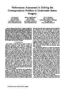
Mean Location Error with SDP Unconstrained versus Genie-aided Edge-Bounding

The algorithm summarized above is what we refer to as a flip-ambiguity-robust SDP-based network localization algorithm with edge-bounding via a Genie. This is in allusion to the fact that in practical situations, the bounds RL and RU , as well as the incidence matrices HU and HL cannot be known. In any case, this theoretical exercise offers insight on the potential of resolving flip-ambiguity through the combination of semidefinite programming and edge-bounding, motivating the feasible solution dealt with in the next subsection. To illustrate, we study the performance of the algorithm summarized by (16) in figures 2 through 4. To this end, define the mean location error for a network of size N with A anchors as

0.045

Unconstrained SDP, α ≤ T Unconstrained SDP, α = 1 SDP with Genie-aided edge-bounding, α ≤ T SDP with Genie-aided edge-bounding, α = 1

0.04

0.035

0.03

ε¯

0.025

0.02

0.015

0.01

0.005

0

ε¯(N ; A)  10

15

20

25

N

Fig. 2.

Mean location error for different α as a function of network size. Mean Location Error with SDP Genie-aided Edge-Bounding: worst case

0.045

Unconstrained SDP, α ≤ T SDP with Genie-aided edge-bounding, α = T 0.04

ε¯

0.035

0.03

0.025

0.02

0.015

10

15

20

25

N

Fig. 3. Mean location error for unconstrained SDP in the least ambiguous scenario (α = 1) versus SDP with Genie-aided edge-bounding in the most ambiguous scenario (α = T ). CDF of Mean Location Error (N = 15) Unconstrained versus Genie-aided Edge-Bounding 1

0.9

0.8

0.7

Pr{ε < ε¯}

0.6

0.5

0.4

0.3

SDP with Genie-aided edge-bounding, α = 1 SDP with Genie-aided edge-bounding, α ≤ T SDP with Genie-aided edge-bounding, α = T Unconstrained SDP, α = 1 Unconstrained SDP, α ≤ T

0.2

0.1

0

0

0.01

0.02

0.03

0.04

ε¯

0.05

0.06

0.07

0.08

Fig. 4. Cumulative density function of the mean location error for different number of α.

ˆ − X X , N −A

(17)

ˆ is the estimate of X. where X Next, we compare in figure 2 the mean location error as a function of the network size obtained with the unconstrained SDP algorithm of (8) against the corresponding error obtained with its flip-ambiguity-robust counterpart. Two curves are shown for each technique, one representing the average situation (α ≤ T ), where any number of target nodes may be subject to flip-ambiguity, and another representing the best possible situation (α = 1), where only one target node is not localizable (see section II). Notice that the location error generally decreases with the network size, which is explained by the fact that the probability of a large number of flip-ambiguous nodes α → T decreases with N (see section II). In any case, the figure clearly demonstrates that the (potential) improvement provided by the edge-bounding technique is very substantial. This can be better illustrated by comparing the performances of the unconstrained SDP in the average situation (α ≤ T ) against the edge-bounded SDP in the worst cases (α = T ), which is done in figure 3. Finally, in figure 4, we compare the cumulative density functions (CDF’s) of the mean location error ε¯ obtained with the unconstrained and ambiguity-robust solutions, for a fixed network size. The figure illustrates the fact that in the presence of scenarios with flip-ambiguity, the performance obtained with the edge-bounded SDP in typical conditions is close to that obtained in the best-possible non-uniquely localizable conditions, that is, when only one target node is flip-ambiguous. In contrast, the unconstrained SDP performs nearly as bad, regardless regardless of the number of flipambiguous target nodes. As a final remark to this section, we point out that the edge-bounded SDP-based flip-ambiguity-robust localization algorithm does not turn a non-uniquely localizable network into a uniquely localizable one, since the solution of obtained from (16) does not lye generally on the η dimensional space. Instead, what occurs is that a solution is obtained in a space of higher dimension, but whose projection onto the ηdimensional space is less likely to exhibit flipped estimates

978-1-4244-4148-8/09/$25.00 ©2009 This full text paper was peer reviewed at the direction of IEEE Communications Society subject matter experts for publication in the IEEE "GLOBECOM" 2009 proceedings.

Mean Location Error with SDP Genie-aided Edge-Bounding versus Fully Constrained + SMACOF

of node locations. Notice that this is not uncommon in SDPbased approaches, as discussed in detail e.g. in [5]. The fact that the solutions of (16) do not generally lye in Rη×T is reflected on the non-zero location errors, which are encountered despite the assumptions of perfect distance estimates (for the distances that are measured). IV. L OCALIZATION WITH S HORTEST- PATH E DGE - BOUNDING

0.02

SDP fully constrained, α ≤ T SDP with Genie-aided edge-bounding, α ≤ T SDP fully constrained + SMACOF, α ≤ T

0.018

0.016

0.014

ε¯

0.012

The results in the preceding section, obtained with the SDP network localization augmented by constraints on a few additional unmeasured distances d˜ij illustrated the remarkable potential of the edge-bounding approach, but are obviously impractical since the information required, specifically d˜ij and RU , cannot be obtained in practice. Inspired by those results, we now set out to design an algorithm that captures the essence of the edge-bounding approach and is implementable. To this end, we introduce the additional constraints not only to a few, but to all unmeasured distances and replace the constant and unknown tight upper-bound RU by the shortest paths between any two points whose distance was not measured. This leads to

0.01

0.008

0.006

0.004

0.002

0

10

15

20

25

N

Fig. 5. Mean location error as a function of network size for SDP with Genie-aided edge-bounding versus Fully constrained SDP and versus Fully constrained SDP+SMACOF.

maximize 0 subject to Z1:η,1:η = Iη

CDF of Mean Location Error (N = 15) Genie-aided Edge-Bounding versus Fully Constrained + SMACOF 1

tr(CT Z) = d2ij , tr(CA Z) = d2kj ,

0.9

0.9

RL2 < tr C†T Z ≤ d†2 ij ,   RL2 < tr C†A Z ≤ d†2 kj , ..................... Z  0,

0.8

0.8

(18)

where d†kj and d†ij are the shortest-path distances from the k-th anchor to the j-th target node, and between the i-th and the j-th target nodes, respectively. Let HF be the incidence matrix corresponding to the fully connected network. It follows ⎤ ⎡ † 0 H 0 T ⎦, H†  HF − HL = ⎣ (19) 0 E†A E†T 

0[η×1]  † †T , (20) CT  0 e [1×η] ij e†ij 

ak  † CA  , (21) aTk e†T † j ej where e†ij is the column vector of E†T whose i-th and j-th elements are 1 and −1, respectively, while e†j is the column vector of E†A whose j-th element is −1. The performance of the algorithm described above can be further improved by feeding the solution obtained from the semidefinite program given in (18) into a good steepestdescent algorithm. This relates to the remark made on the last paragraph of the preceding section and results from the fact that the semidefine solution does not lye in η-dimensional

0.7

0.7

0.6 0.6

Pr{ε < ε¯}

....... . . . . . . ........

0.5 0.4

0.5

0.3 0.4

0.2 0.1

0.3

0 0.2

0.005

0.01 0.015

0.02 0.025

SDP fully constrained + SMACOF, α ≤ T SDP with Genie-aided edge-bounding, α ≤ T SDP fully constrained, α ≤ T

0.1

0

0

0

0.01

0.02

0.03

0.04

0.05

ε¯

0.06

0.07

0.08

0.09

0.1

Fig. 6. Cumulative density function of the mean location error for realizations of SDP and, inside the inner rectangle, a closer-up view of the curves.

space (see [5] and references thereby). Here we select the SMACOF [10] for such a “refining” algorithm. In figure 5 we compare the mean location error obtained from (18), both with and without SMACOF-based refining against that of the algorithm described in section III. Unsurprisingly, it is found that the performance of the “raw” SDPbased solution is slightly worse than that of the algorithm with a Genie. It is remarkable, however, that the performance of the feasible technique is not far off from the unfeasible one. Furthermore, it can the seen that the performance of the feasible solution after refinement via SMACOF is in fact better than that of the algorithm with a Genie and no refinement.

978-1-4244-4148-8/09/$25.00 ©2009 This full text paper was peer reviewed at the direction of IEEE Communications Society subject matter experts for publication in the IEEE "GLOBECOM" 2009 proceedings.

Finally, the CDF’s of the mean location errors corresponding to the three schemes compared in figure 5 are plotted in figure 6. This final figure reveals that, in percentile terms, the feasible variation of the edge-bouded SDP-based network localization algorithm with flip-ambiguity robustness is, to all effect, as good as the Genie-aided counterpart, and that the complete solution (including SMACOF refining) is even better. Figure 6 also shows that in over 80% of trials, for instance, the proposed technique is capable of maintaining the mean location error at the fraction of 1% of the largest dimension of the network, despite the flip-ambiguity problem that afflicts the networks studied.

[8] D. Moore, J. Leonard, D. Rus, and S. Teller, “Robust Distributed Network Localization with Noisy Range Measurements,” in IEEE Proceedings of the 2nd international conference on Embedded networked sensor systems (SenSys04), 2004, pp. 50–61. [9] L. E. Miller, “Distribution of Link Distances in a Wireless Network,” Journal of Research of the National Institute of Standards and Technology, vol. 106, pp. 401–412, 2001. [10] T. F. Cox and M. A. A. Cox, Multidimensional Scaling, 2nd ed. Chapman & Hall/CRC, 2000. [11] G. Destino, G. Abreu, “Weighing Strategy for Network Localization under Scarce Ranging Information,” IEEE Transactions on Wireless Communications, p. (submitted), 2009.

V. C ONCLUSION We employed the unique localizability test recently proposed in [4] to study the problem of flip-ambiguity in network localization and motivate a novel formulation of the SDP localization algorithm that is robust to flip-ambiguity. To the best of the authors’ knowledge, this marks a departure from the dominant approach to handle the problem found in current, which is to avoid, rather than resolve, flipambiguities. As a first in its approach, the work is preliminary, but also inspiring and insightful, in which it demonstrates the feasibility of concrete flip-ambiguous solutions with excellent performance. One topic for future work is the extension of the result through the application of the strong localizability test so as to better capture the effect of small perturbations on the node locations and their mutual distances. One further step under consideration is the formulation of a similar approach with basis on a simpler steepest-descent optimization method, for example by translating the edge-bounding technique onto an equivalent weighing strategy [11]. R EFERENCES [1] N. B. Priyantha, H. Balakrishnan, E. D. Demaine, and S. J. Teller, “Anchor-Free Distributed Localization in Sensor Networks.” in ACM Conference on Embedded Networked Sensor Systems (SenSys 2009). ACM, 2003, pp. 340–341. [2] N.-H. Z. Leung and K.-C. Toh, “An SDP-based divide-and-conquer Algorithm for large Scale noisy Anchor-free Graph realization,” 2008, PrePrint. [3] A. Kannan, B. Fidan, G. Mao, and B. Anderson, “Analysis of Flip Ambiguities in Distributed Network Localization,” in Information, Decision and Control, 2007. IDC ’07, Feb. 2007, pp. 193–198. [4] A. M. So and Y. Ye, “Theory of Semidefinite Programming for Sensor Network Localization,” in Proc. IEEE Sixteenth Annual ACMSIAM Symposium on Discrete Algorithms (SODA), Vancouver, British Columbia Canada, January 2005, pp. 405–414. [5] P. Biswas, T.-C. Liang, K.-C. Toh, and T.-C. Wang, “Semidefinite Programming Based Algorithms for Sensor Network Localization with noisy Distance Measurements,” ACM Transactions on Sensor Networks (TOSN), vol. 2, no. 2, pp. 188–220, May 2006. [6] P. Biswas and Y. Ye, “A Distributed Method for Solving Semidefinite Programs Arising from Ad Hoc Wireless Sensor Network Localization,” Tech. Rep., 2003. [7] A. Kannan, B. Fidan, and G. Mao, “Robust Distributed Sensor Network Localization based on Analysis of Flip Ambiguities,” in Proc. IEEE Global Telecommunications Conference (GLOBECOM 2008), December 2008, pp. 1–6.

978-1-4244-4148-8/09/$25.00 ©2009 This full text paper was peer reviewed at the direction of IEEE Communications Society subject matter experts for publication in the IEEE "GLOBECOM" 2009 proceedings.