1340
IEEE TRANSACTIONS ON NEURAL NETWORKS, VOL. 19, NO. 8, AUGUST 2008
A Novel Recurrent Neural Network for Solving Nonlinear Optimization Problems With Inequality Constraints Youshen Xia, Senior Member, IEEE, Gang Feng, Senior Member, IEEE, and Jun Wang, Fellow, IEEE
Abstract—This paper presents a novel recurrent neural network for solving nonlinear optimization problems with inequality constraints. Under the condition that the Hessian matrix of the associated Lagrangian function is positive semidefinite, it is shown that the proposed neural network is stable at a Karush–Kuhn–Tucker point in the sense of Lyapunov and its output trajectory is globally convergent to a minimum solution. Compared with variety of the existing projection neural networks, including their extensions and modification, for solving such nonlinearly constrained optimization problems, it is shown that the proposed neural network can solve constrained convex optimization problems and a class of constrained nonconvex optimization problems and there is no restriction on the initial point. Simulation results show the effectiveness of the proposed neural network in solving nonlinearly constrained optimization problems. Index Terms—Global convergence, nonconvex programming, nonlinear inequality constraints, nonsmooth analysis, recurrent neural network.
I. INTRODUCTION
A
NONLINEARLY constrained optimization problem is to minimize a nonlinear objective function subject to linear and nonlinear constraints. If the objective function and constraints are linear, the problem is a linear program. Otherwise, it is called a nonlinear program. Many engineering problems, such as optimal control, structure design, mechanical design, and electrical networks planning, can be formulated as constrained nonlinear optimization problems [1]. Numerical optimization procedures have been presented over decades for solving nonlinear convex optimization problems (see [1]–[5], and the references therein). In many applications, real-time solutions are usually imperative [6]. As a software and hardware-implementable approach [7], recurrent neural networks for solving linear and nonlinear constrained optimization problems have been developed in the last decade. Compared with traditional numerical optimization algorithms, the neural network approach has several potential advantages in real-time
Manuscript received December 3, 2006; revised September 7, 2007; accepted January 6, 2008. First published May 7, 2008; last published August 6, 2008 (projected). Y. Xia is with the College of Mathematics and Computer Science, Fuzhou University, China (e-mail:
[email protected]). G. Feng is with the Department of Manufacturing Engineering and Engineering Management, The City University of Hong Kong, Hong Kong (e-mail:
[email protected]). J. Wang is with the Department of Automation and Computer-Aided Engineering, The Chinese University of Hong Kong, New Territories, Hong Kong, China (e-mail:
[email protected]). Digital Object Identifier 10.1109/TNN.2008.2000273
applications. First, the structure of a neural network can be implemented effectively using very large scale integration (VLSI) and optical technologies. Second, neural networks can solve many optimization problems with time-varying parameters. Third, the dynamical techniques and the numerical ODE techniques can be applied directly to the continuous-time neural network for solving constrained optimization problems effectively. In addition, recent reported results have shown that the global convergence of the recurrent neural network approach to nonlinearly constrained convex optimization problems can be achieved under weaker conditions than the conventional numerical optimization algorithm. For example, no Lipschitz condition is required for the recurrent neural network approach. Tank and Hopfield proposed first in 1986 [8] a neural network for linear programming that was mapped onto a closed-loop circuit. Kennedy and Chua extended [9] the Tank–Hopfield network by developing a neural network with a finite penalty parameter for solving nonlinear convex programming problems. Although their network actually fulfills both the Kuhn–Tucker optimality conditions in terms of penalty function, this network is not capable of finding an exact optimal solution due to a finite penalty parameter and is difficult to implement when the penalty parameter is very large [10]. Variety of attempts to avoid using penalty parameters have been made. For example, Rodriguez-Vazquez et al. [11] proposed a switched-capacitor neural network for solving a class of constrained nonlinear convex optimization problems. This network is suitable for the case that the optimal solutions lie in the interior of the feasible region. Otherwise, the network may have no equilibrium point [12]. Zhang and Constantinides developed [13] a Lagrange neural network for a nonlinear programming problem with equality constraints. Bouzerdoum and Pattison [14] presented a recurrent neural network for solving convex quadratic optimization problems with bounded constraints only. Xia [15], [16] presented two recurrent neural networks for solving linear and quadratic convex programming problems and nonlinear convex optimization problems with limit constraints. Liang and Wang [17] presented a recurrent neural network for nonlinear convex optimization with bounded constraints. Xia et al. [18] developed a projection neural network for solving monotone variational inequality problems with limit constraints. By extending projection neural network, Xia and Wang [20], [21] developed two recurrent neural networks for solving strictly convex programming with nonlinear inequality constraints and linear constraints, respectively. Hu and Wang studied how to use the projection neural network to solve pseudomonotone variational inequality problems. Recently, Xia and Feng [24]
1045-9227/$25.00 © 2008 IEEE
XIA et al.: NOVEL RECURRENT NEURAL NETWORK FOR SOLVING NONLINEAR OPTIMIZATION PROBLEMS
introduced another projection-type neural network for solving a class of monotone projection equations. However, many real-world constrained optimization problems may be nonconvex [25], [26]. As a result, recurrent neural networks for solving nonconvex optimization problem have been also studied. For example, two neural network models for unconstrained nonconvex optimization were presented in [27] and [28], and a neural network model for nonconvex quadratic optimization was presented in [29]. The objective of this paper is to develop a novel neural network model for solving nonlinear constrained optimization problems with nonlinear inequality constraints. It is shown that under the condition that the Hessian matrix of the associated Lagrangian function is positive semidefinite, the proposed neural network is stable at a Karush–Kuhn–Tucker point in the sense of Lyapunov and its output trajectory is globally convergent to a minimum solution. Compared with the existing switched-capacitor neural network, the proposed neural network has no requirement on the optimal solution, which lies in the interior of the feasible region. Compared with the existing projection neural networks including their extensions [20]–[23], the proposed neural network can be guaranteed to solve constrained convex programming problems and a class of constrained nonconvex programming problems without restriction on the initial point. Simulation results show that the proposed neural network is indeed effective in solving nonlinearly constrained programming problems. This paper is organized as follows. In Section II, the nonlinearly constrained optimization problem and its equivalent formulations are described. In Section III, a recurrent neural network model is proposed to solve such nonlinear optimization problems, and a comparison with existing approaches is given. In Section IV, the global convergence of the proposed neural network is analyzed. In Section V, simulation results are presented to evaluate the effectiveness of the proposed neural network. Finally, Section VI concludes this paper.
1341
is nonempty and bounded, then the NOP has at least one ophas timal solution. While the feasible set is unbounded but a bounded level set, the NOP has also an optimal solution [31]. From [1], we know that if , which is feasible and regular, is a local optimal solution of the NOP, then there exists such that is a Karush–Kuhn–Tucker (KKT) point satisfying
(2) where and is the gradient of . By the well-known projection theorem [2], we know that the KKT condition defined in (2) can be rewritten as two projection equations (3) where
, ,
if and only if and let
, and . That is, is a KKT point satisfies (3). Furthermore, let
Then, is a KKT point if is also a solution of the following variational inequality problem: (4)
III. NEURAL NETWORK MODEL In [16], to solve the following convex programming problem:
II. PROBLEMS AND FORMULATION
minimize
In this section, we describe nonlinearly constrained optimization problem and discuss its equivalent formulations. Consider the following nonlinear optimization problem (NOP):
subject to
(5)
where is convex and differentiable, a neural dynamical approach, called an ODE method, was developed as follows: state equation
(6)
output equation minimize
subject to
(1)
, is where an -dimensional vector-valued continuous function of variare assumed to be twice ables, and the functions differentiable. In optimization literature, NOP is called the nonand are all convex, linear programming problem. If the NOP is called a convex programming problem (CPP). Otherwise, the NOP is called a nonconvex programming problem (NCPP). A vector is called a feasible solution to the NOP if and only if satisfies the constraints of the NOP and nonnegative constraints. The feasible solution is said to be a regular , , , point if the gradients of are linearly independent. When the set of all feasible solutions
where is the state trajectory of (6), is its output trajec, and . tory, It was shown in [16] that the output trajectory of this approach converges globally to an optimal solution of (5). In this paper, by extending the aforementioned model structure defined in (6), we propose the following recurrent neural network model for solving the NOP: state equation
(7) output equation
1342
IEEE TRANSACTIONS ON NEURAL NETWORKS, VOL. 19, NO. 8, AUGUST 2008
where is the state trajectory of the proposed neural is its output trajectory, and is a network in (7), designing constant. The dynamical state equation described by (7) can be easily realized by a recurrent neural network with a one-layer structure. The circuit realizing the proposed integrators, piecewise neural network consists of and , processors for linear activation functions for , processors for , processors for , and some summers. Therefore, the proposed network complexity and as well as only depends on the mapping in the original problem. To see the advantages of the proposed neural network model, we compare it with the existing neural network models for solving (1). First, Kennedy and Chua proposed [9] the following neural network model for solving the NCOP:
the NCOP with strict convex objective function and the NCOP, respectively, in [20]–[22]. The extended projection neural network can be used to solve pseudoconvex NOPs but the initial [22], [30]. We will show that the point has to satisfy proposed neural network can solve both the NCOP and a class of nonconvex NOPs without a limitation on the initial point. Fi, the proposed neural netnally, in a special case that work model (7) will reduce to (6). Thus, the proposed neural network model can generalize the existing neural network model (6). Finally, we compare the proposed neural network algorithm with the existing related numerical algorithms for solving (1). First, consider the modified projection-type algorithm [4], which is defined as (12)
(8) and
where where is a penalty parameter. This model has a smaller size than (7) but it cannot converge to an exact optimal solution of the NCOP due to the penalty parameter. Rodriguez-Vazquez et al. [11] developed the following switched-capacitor neural network model for solving the NCOP:
, and
are scaling parameters, , , , and
if (9) if where
, and . The switched-capacitor neural network model also has smaller size than (7). However, it needs to compute a per iteration when the trajectory time-varying index set . Thus, the proposed neural network model is more suitable for implementation than the switched-capacitor neural network model. Moreover, for the global convergence, the switched-capacitor neural network requires the condition that is bounded and the optimal solution the feasible region must lie in the interior of , whereas the proposed neural network will be shown to be globally convergent without these conditions. Recently, based on a projection neural network model [18], several recurrent neural networks were developed for solving various constrained convex optimization problems, respectively, in [19]–[21]. The extended projection neural network models for solving (1) can be described by (10) It is easy to see that the extended projection neural network model (10) has the same network complexity with the proposed neural network model (7). In addition, there exists a neural network model [23] for solving (1), defined by
On one side, the modified projection-type method is not suitable for parallel implementation due to the choice of the varying step . Also, the modified projection-type method is relength , , quired to compute additional nonlinear terms per iteration, and thus has higher computational comand plexity. On the other side, the global convergence of the modified projection-type method is guaranteed only when the NP problem (1) is convex programming and the following Lipschitz condition:
and are satisfied, while the proposed neural network will be shown to converge globally without requiring the Lip. It is worth pointing out that schitz condition and is nonlinear, the aforementioned Lipschitz condition when is difficult to be satisfied. As a result, the global convergence of the projection-type algorithm cannot be guaranteed for such cases. In addition, there are some other methods for solving nonconvex nonlinear programming problems, respectively, based on the primal–dual technique [31] and the scaling technique [32]. In comparison with these approaches, the proposed neural network approach has a lower computational complexity and requires weaker conditions for global convergence. IV. STABILITY ANALYSIS
(11) This neural network model actually is a modification of the extended projection neural network model (10) by replacing the . As a result, the neural netvariable by term work model (11) has a two-layer projection structure and thus has higher network complexity than both (7) and (10). Theoretically, the neural networks in (10) and (11) were shown to solve
In this section, we discuss the global convergence of the proposed neural network for solving the NOP. We first give the following definitions and lemmas. of For convenience of discussion, the Hessian matrix is said to be positive semidefinite at if
XIA et al.: NOVEL RECURRENT NEURAL NETWORK FOR SOLVING NONLINEAR OPTIMIZATION PROBLEMS
and is positive definite at . equality holds whenever if semidefinite on a set
if the previous strict inis said to be positive
is positive definite on the set if the strict inequality . holds in the previous equation whenever A Lagrangian function associated with the NOP is defined as
1343
That is
Thus, is a solution of (3) and hence is a KKT point. Lemma 3: For any , , we have (13)
Its Hessian matrix is then given by . We denote the KKT point of the NOP by , the set of minimizers of the NOP by , and the state . trajectory of (7) by Throughout this paper, we assume that the NOP has at least a local optimal solution. Lemma 1 [2]: Let be a closed convex set. Then
where , defined in (13) is shown in the equation at the bottom of the page, and if if Proof: Let prove that for
. It is enough to
and There are four cases to be considered. First, let . Then, due to Thus where denotes is defined by
and .
norm and the projection operator
Lemma 2: i) For any initial point , there exists for (7) over . Specially, a unique continuous solution is bounded, . ii) The equilibrium set of (7) is when is an equilibrium point of nonempty. Moreover, if is a KKT point. (7), then Proof: , , and are locally Lipsi) Since chitz continuous, so is the right-hand side of (7). According to the local existence theorem of ordinary differential equations, there exists a unique continuous solution of (7) for . trajectory ii) Since the NOP has a local minimizer , by the KKT such that theorem, we know that there exists is a KKT point satisfying (3). Let be defined in (4). Then, it can be verified that is an equilibrium point of (7). Thus, the equilibrium set is the equilibrium of (7) is nonempty. Next, if point of (7), then
.. .
and . Thus, Next, let Without loss of generality, we assume that there exists such that for and for . Then
since holds for the case that . Then, Thus
(14) .
. Hence, we have (14). Similarly, (14) and . Finally, let and due to .
which implies that (14) holds as well. Therefore, the conclusion of Lemma 3 is obtained. According to the second-order necessary condition, we see is a local optimal solution; then, there exists so that that the Hessian matrix must be positive semidefinite.
.. .
..
.
.. .
1344
IEEE TRANSACTIONS ON NEURAL NETWORKS, VOL. 19, NO. 8, AUGUST 2008
Based on this observation, we begin to establish our main results on concerning the global convergence of the proposed neural network. as the second For convenience of description, we define state trajectory of (7) with zero initial point, and define an associated set , where is a nonzero vector. is positive semidefinite Theorem 1: Assume that and is positive definite. For any initial point on , if is positive semidefinite on , then the proposed neural network is stable at a KKT point and its output trajectory converges globally to a minimum solution of the NOP. be the state trajectory of Proof: Let . Consider the Lyapunov (7) with the initial point function
(15) where Clearly,
It follows that is differentiable and is arbitrary. Now, from Lemma 1, we know that
since
Then
Since
is also a solution of (4)
It follows that
,
, , is a KKT point. . It is easy to see that for any On one side, by applying the mean-value theorem [31] to defined in (4), we have for any
According to Lemma 3, we see that for any
where is a symmetric matrix. Thus, similar to analysis given in [33, p. 96], we have
It follows that
Taking
for
sufficiently small, we have
where
where
is a zero matrix. Let . Then
and
where and . Note that the second state trajectory of (7) with the nonzero initial can be expressed as . point The equation shown at the bottom of the next page holds since is positive semidefinite on ; so the proposed neural network in (7) is stable at . Because of and , is monotone, the monotonicity of functions is convex in . Note that and is and thus, and the level set a global minimizer of . Then, is bounded and the solution trajectory is bounded due to . It follows from LaSalle’s
XIA et al.: NOVEL RECURRENT NEURAL NETWORK FOR SOLVING NONLINEAR OPTIMIZATION PROBLEMS
invariance principle that the trajectories will converge to , the largest invariant subset of the following set:
That is, plies that
where . Since
. Note that
im-
and and are continuous and is positive semidefinite
In particular, when
It follows that positive definite. Thus
,
and
1345
is positive definite. Therefore, the output trajectory of the proposed neural network converges globally to a minimum solution of the NOP. It is well known that studying the convergence rate of the neural network is useful [34], [35]. As for the convergence rate of the proposed neural network, we have the following result. Theorem 2: Assume that is positive definite on . For any initial point , if is positive semidefinite on , then the convergence rate of the proposed neural network is proportional to a design parameter in the sense described by
(16) is a constant proportional to . where is positive Proof: First, since , for each , the Lagrange function is definite on strictly monotone with respect to . Thus, there exists only one satisfying
. Then
since
is
Hence, the NOP has only one local optimal solution. Next, let be the state trajectory of the proposed neural . Consider the function denetwork with the initial point fined in Theorem 1
so Then, for any given 1, we see that
, from the analysis of Theorem
Therefore, the output trajectory of the proposed neural network globally converges to the set of the minimizers of the NOP. Spe, then cially, if the set
Finally, according to the second-order sufficiency condition, must be a local optimal solution of the NOP since
(17)
1346
IEEE TRANSACTIONS ON NEURAL NETWORKS, VOL. 19, NO. 8, AUGUST 2008
In particular, the above inequality still holds when . , then we That is, let have
and
. It follows that
It can be verified that
On one side, let so we have
Then, set as being bounded and closed, and . Since is positive definite , so is on . on Then
Thus, there exists
Let . It follows (16). Corollary 1: Assume that is differentiable and pseudoand is positive definite. For any initial convex on point, the neural network in (6) is stable in the sense of Lyapunov and its output trajectory converges to an optimal solution of (5). Proof: Consider the Lyapunov function
such that (18)
Hence
It follows that
On the other side, we have
From Lemma 1, we can obtain that for any
where , , and is an optimal solution of (5). Similar to the analysis of Theorem 1, we know is differentiable and . Then that
Because is differentiable and pseudconvex on is pseudmonotone on . That is
,
Thus, . It follows from LaSalle’s invariance prinof (6) will converge to . ciple that the state trajectories can By Theorem 1, we know that the positiveness of . Thus, the output trajectory of (6) imply that will converge to . Finally, we illustrate the significance of obtained results. First, when the NOP is the CPP, the Kuhn–Tucker conditions are then the sufficient conditions for to be a global optimal solution to the NOP. By Theorem 1, we see that the proposed neural network can solve constrained convex optimization problems and the CPP since the Lagrangian multiplier is always nonnegative. Second, the condition that vector is positive semidefinite allows or some may not be positive that either semidefinite. As a result, the proposed neural network can be used to solve such a class of the NCPP with the KKT point corresponding to the global optimal solution of the NCPP. For is convex and some constraint example, in one case that
XIA et al.: NOVEL RECURRENT NEURAL NETWORK FOR SOLVING NONLINEAR OPTIMIZATION PROBLEMS
1347
Fig. 1. Transient behavior of state trajectory (x (t); x (t)) based on (7) with 100 random initial points in Example 1.
function is concave, if the feasible set is convex, then the proposed neural network can be used to solve this class of is nonconvex optimization problems. In another case that are convex, then the nonconvex while constraint functions proposed neural network can also be used to solve this class of nonconvex programming problems. In particular, compared with the results on the global convergence of the extended projection neural network, the proposed neural network has no re. striction on the initial point Remark 1: It should be noted that when is differentiable, the following equality
is the classic result on symmetric gradient mapping in [33, page 95-96]. In this paper, is nondifferentiable, so our result on the previous equality in this paper actually generalizes the classic result. As a result, the stability analysis of the proposed neural network is different from that of the existing projection neural networks and their extensions [15]–[24], [30]. Remark 2: Let us consider an extension of the NOP minimize
subject to
(19)
, , and . Directly extending (7), we have the following neural network for solving (19): where
state equation
(20) output equation
where
and
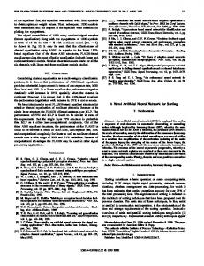
Similarly to Theorems 1 and 2, we can obtain the global convergence results on (20). V. ILLUSTRATIVE EXAMPLES In this section, several illustrative examples are discussed to demonstrate the effectiveness of the proposed neural network. Example 1: Consider the following convex programming problem minimize subject to where
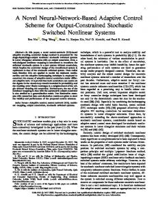
and . This problem has a unique solution , where and are all convex. We use the proposed neural network to solve the aforementioned problem. All simulation results show that the output state trajectory of (7) with any initial point is always convergent to . For example, . Fig. 1 displays the transient behavior of state trajeclet based on (7) with 100 random initial points, tories and Fig. 2 displays the transient behavior of output trajectories based on (7) with the same initial points. From Figs. 1 and 2, we can see that although both the state and output trajectories converge to the optimal solution, the output trajectory has a faster convergence rate. For comparison, we further tested the existing algorithms: the extended projection neural
1348
IEEE TRANSACTIONS ON NEURAL NETWORKS, VOL. 19, NO. 8, AUGUST 2008
Fig. 2. Transient behavior of output trajectory (v (t); v (t)) based on (7) with same random initial points in Example 1.
TABLE I COMPUTED RESULTS OF THREE METHODS IN EXAMPLE 1
network (PNN) algorithm defined in (10) and modified projection-type (MPT) algorithm described in (12), where and . Table I gives their computational results under different initial points. It shows that the proposed neural network has a better performance in convergence time and solution accuracy than the PNN algorithm and the MPT algorithm. Example 2: Consider the following quadratic fractional problem:
minimize subject to
where
,
, and
This example comes from [22], but here the set is different and this problem has an optimal solution . The objective function is pseudoconvex on . The existing convergence results [16]–[21] cannot ensure the global convergence to the optimal solution. However, Corollary 1 guarantees that the proposed neural network is convergent to . We now apply the proposed neural
XIA et al.: NOVEL RECURRENT NEURAL NETWORK FOR SOLVING NONLINEAR OPTIMIZATION PROBLEMS
1349
Fig. 3. Convergence behavior of the output trajectory norm error based on (7) with five random initial points in Example 2.
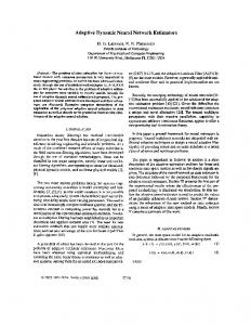
Fig. 4. Behavior of the state projection trajectory of (7) with zero initial point in Example 3.
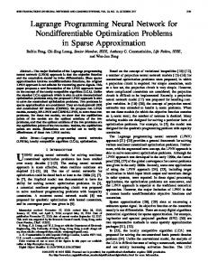
network to solve the aforementioned pseudoconvex optimization problem. Simulation results show that the output trajectory of the proposed neural network is always convergent to . For
. Fig. 3 displays the transient behavior of the example, let based on the proposed output trajectory norm error neural network with five random initial points.
1350
IEEE TRANSACTIONS ON NEURAL NETWORKS, VOL. 19, NO. 8, AUGUST 2008
Fig. 5. Convergence behavior of the output trajectory norm error based on (7) with five random initial points in Example 3.
Fig. 6. Behavior of the state projection trajectory of (7) with zero initial point in Example 4.
Example 3: Consider the following nonconvex programming problem [26]: minimize subject to
(21)
where and . is convex but is not convex. This problem has an optimal solution
and the corresponding optimal Lagrangian multiplier . Because is nonconvex, the existing neural networks [19]–[21] could not guarantee their convergence to . Now, we apply the proposed neural network in (7) to the nonconvex programming problem. Let . Fig. 4 shows that the state projection trajectory of (7) with zero initial point is always less than . Note that for any
XIA et al.: NOVEL RECURRENT NEURAL NETWORK FOR SOLVING NONLINEAR OPTIMIZATION PROBLEMS
1351
TABLE II COMPUTED RESULTS OF TWO ALGORITHMS UNDER THE SAME INITIAL POINTS IN EXAMPLE 3
TABLE III RESULTS FOR THREE METHODS WITH DIFFERENT INITIAL POINTS IN EXAMPLE 4
Furthermore, we compare the proposed neural network algorithm with the nonlinear numerical optimization (NNO) algorithm based on MATLAB software. Table II gives their computed results under different initial points, which show that the proposed neural network has a better performance in convergence time and solution accuracy than the NNO algorithm. Example 4: Consider the following nonconvex programming problem:
minimize subject to where
and
, the associated state projection . Thus, it will be .
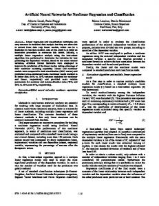
This problem has an optimal solution (with accuracy up to four digits). The corresponding optimal . Because is Lagrangian multiplier nonconvex, the existing neural networks [19]–[21] could not guarantee their convergence to . Now, we apply the proposed neural network in (7) to the nonconvex programming problem. Fig. 6 first displays the state projection trajectory of (7) with zero initial point. It is easy to see that when . As a result, for any given nonzero initial point , the associated state projection trajectory will be larger than when . Thus
is positive definite for . Theorems 1 and 2 guarantee that the output trajectory of the proposed neural network in (7) converge globally to . For example, let . Fig. 5 displays the transient behavior of the output trajectory norm error based on (7) with five random initial points.
is positive definite for . Thus, Theorem 1 guarantees that the output trajectory of the proposed neural network can converge globally to . Simulation results show that the output trajectory of the proposed neural network is always convergent to . For example, let . Fig. 7 displays the transient
given nonzero initial point trajectory less than six when Hence
1352
IEEE TRANSACTIONS ON NEURAL NETWORKS, VOL. 19, NO. 8, AUGUST 2008
Fig. 7. Convergence behavior of the output trajectory norm error based on (7) with five random initial points in Example 4.
behavior of the output trajectory norm error based on (7) with five random initial points. Furthermore, we compare the proposed neural network with the existing extended projection neural network (EPNN) defined in (10) and the modified projection neural network (MPNN) defined in (11) in solving this problem. Simulation results show that the trajectory of EPNN and the MPNN (4) could not converge to except for those initial points that are closer to , whereas the proposed neural network always converges to whether the initial point is very close to or not. For example, let . Table I listed computed results of three neural networks.
VI. CONCLUDING REMARKS In this paper, we proposed a recurrent neural network for solving general nonlinear optimization problems subject to nonlinear inequality constraints, by extending the structure of a novel neural network model. The equilibrium points of the proposed neural network are found to correspond to the KKT point associated with the nonlinearly constrained optimization problem. The global convergence of the proposed neural network is proved under the condition that the Hessian matrix of the associated Lagrangian function is positive semidefinite. Compared with the existing projection neural networks, including their extensions, for solving such nonlinearly constrained optimization problems, it is shown that the proposed neural network can solve constrained convex optimization problems and a class of constrained nonconvex optimization
problems and there is no restriction on the initial point. Simulation results have shown that the proposed neural network is effective in solving nonlinearly constrained optimization problems.
REFERENCES [1] M. S. Bazaraa, H. D. Sherali, and C. M. Shetty, Nonlinear Programming: Theory and Algorithms, 2nd ed. New York: Wiley, 1993. [2] D. Kinderlehrer and G. Stampcchia, An Introduction to Variational Inequalities and their Applications. New York: Academic, 1980. [3] F. Facchinei, A. Fischer, and C. Kanzow, “A simply constrained optimization reformulation of KKT systems arising from variational inequalities,” Appl. Math. Optim., vol. 40, pp. 19–37, 1999. [4] M. V. Solodov and P. Tseng, “Modified projection-type methods for monotone variational inequalities,” SIAM J. Control Optim., vol. 2, pp. 1814–1830, 1996. [5] A. Wachter and L. T. Biegler, “Line search filter methods for nonlinear programming: Motivation and global convergence,” SIAM J. Optim., vol. 16, pp. 1–31, 2005. [6] N. Kalouptisidis, Signal Processing Systems, Theory and Design. New York: Wiley, 1997. [7] A. Cichocki and R. Unbehauen, Neural Networks for Optimization and Signal Processing. London, U.K.: Wiley, 1993. [8] D. W. Tank and J. J. Hopfield, “Simple ’neural optimization networks: An A/D converter, signal decision circuit, and a linear programming circuit,” IEEE Trans. Circuits Syst., vol. CAS-33, no. 5, pp. 533–541, May 1986. [9] M. P. Kennedy and L. O. Chua, “Neural networks for nonlinear programming,” IEEE Trans. Circuits Syst., vol. CAS-35, no. 5, pp. 554–562, May 1988. [10] W. E. Lillo, M. H. Loh, S. Hui, and S. H. Zak, “On solving constrained optimization problems with neural networks: A penalty method approach,” IEEE Trans. Neural Netw., vol. 4, no. 6, pp. 931–939, Nov. 1993. [11] A. Rodríguez-Vázquez, R. Domínguez-Castro, A. Rueda, J. L. Huertas, and E. Sánchez-Sinencio, “Nonlinear switched-capacitor ’neural networks’ for optimization problems,” IEEE Trans. Circuits Syst., vol. 37, no. 3, pp. 384–397, Mar. 1990.
XIA et al.: NOVEL RECURRENT NEURAL NETWORK FOR SOLVING NONLINEAR OPTIMIZATION PROBLEMS
[12] M. P. Glazos, S. Hui, and S. H. Zak, “Sliding modes in solving convex programming problems,” SIAM J. Control Optim., vol. 36, pp. 680–697, 1998. [13] S. Zhang and A. G. Constantinides, “Lagrange programming neural networks,” IEEE Trans. Circuits Syst. II, Analog Digit. Signal Process., vol. 39, no. 7, pp. 441–452, Jul. 1992. [14] A. Bouzerdoum and T. R. Pattison, “Neural network for quadratic optimization with bound constraints,” IEEE Trans. Neural Netw., vol. 4, no. 2, pp. 293–304, Mar. 1993. [15] Y. S. Xia, “A new neural network for solving linear programming problems and its applications,” IEEE Trans. Neural Netw., vol. 7, no. 2, pp. 525–529, Mar. 1996. [16] Y. S. Xia, “ODE methods for solving convex programming problems with bounded variables,” Chin. J. Numer. Math. Appl. (English Edition), vol. 18, no. 1, 1996. [17] X. B. Liang and J. Wang, “A recurrent neural network for nonlinear optimization with a continuously differentiable objective function and bound constraints,” IEEE Trans. Neural Netw., vol. 11, no. 6, pp. 1251–1262, Nov. 2000. [18] Y. S. Xia, H. Leung, and J. Wang, “A projection neural network and its application to constrained optimization problems,” IEEE Trans. Circuits Syst. I, Fundam. Theory Appl., vol. 49, no. 4, pp. 447–458, Apr. 2002. [19] Y. S. Xia, “An extended projection neural network for constrained optimization,” Neural Comput., vol. 16, no. 4, pp. 863–883, 2004. [20] Y. S. Xia and J. Wang, “A recurrent neural network for solving nonlinear optimization subject to nonlinear inequality constraints,” IEEE Trans. Circuits Syst. I, Reg. Papers, vol. 51, no. 7, pp. 1385–1394, Jul. 2004. [21] Y. S. Xia and J. Wang, “A recurrent neural network for solving nonlinear convex programs subject to linear constraints,” IEEE Trans. Neural Netw., vol. 16, no. 2, pp. 379–386, Mar. 2005. [22] X. Hu and J. Wang, “Solving pseudomonotone variational inequalities and pseudoconvex optimization problems using the projection neural network,” , vol. 6, pp. 1487–1499, 2006. [23] X. B. Gao, “A neural network for solving nonlinear convex programming problems,” IEEE Trans. Neural Netw., vol. 15, no. 3, pp. 613–621, May 2003. [24] Y. S. Xia and G. Feng, “A new neural network for solving nonlinear projection equations,” Neural Netw., vol. 20, pp. 577–589, 2007. [25] J. C. Principe, J. M. Kuo, and S. Celebi, “An analysis of the gammamemory in dynamic neural networks,” IEEE Trans. Neural Netw., vol. 5, no. 2, pp. 331–337, Mar. 1994. [26] M. Avriel and A. C. Williams, “An extension of geometric programming with applications in engineering optimization,” J. Eng. Math., vol. 5, pp. 187–1999, 1971. [27] D. Beyer and R. Ogier, “Tabu learning: A neural network search method for solving nonconvex optimization problems,” in Proc. IEEE Int. Joint Conf. Neural Netw., 2000, vol. 2, pp. 953–961. [28] C. Y. Sun and C. B. Feng, “Neural networks for nonconvex nonlinear programming problems: A switching control approach,” in Lecture Notes in Computer Science, ser. 3496. Berlin, Germany: Springer-Verlag, 2005, pp. 694–699. [29] Q. Tao, X. Liu, and M. S. Xue, “A dynamic genetic algorithm based on continuous neural networks for a kind of non-convex optimization problems,” Appl. Math. Comput., vol. 150, pp. 811–820, 2004. [30] Y. S. Xia and G. Feng, “On the convergence condition of the extended projection neural network,” Neural Comput., vol. 17, pp. 515–525, 2005. [31] A. Forsgren and P. E. Gill, “Primal-dual interior method for nonconvex nonlinear programming,” SIAM J. Optim., vol. 8, pp. 1132–1152, 1998. [32] D. Li and X. L. Sun, “Local convexification of the Lagrangian function in nonconvex optimization,” J. Optim. Appl., vol. 104, pp. 109–120, 2000. [33] J. M. Ortega and W. G. Rheinboldt, Iterative Solution of Nonlinear Equations in Several Variables. New York: Academic, 1970. [34] C. Y. Sun and C. B. Feng, “Exponential periodicity and stability of delayed neural networks,” Math. Comput. Simulat., vol. 66, pp. 469–478, 2004.
1353
[35] C. Y. Sun and C. B. Feng, “Exponential periodicity of continuous-time and discrete-time neural networks with delays,” Neural Process. Lett., vol. 19, pp. 131–146, 2004. Youshen Xia (M’96–SM’00) received the B.S. and M.S. degrees in computational mathematics from Nanjing University, Nanjing, China, in 1982 and 1989, respectively, and the Ph.D. degree from the Department of Automation and Computer-Aided Engineering, The Chinese University of Hong Kong, China, in 2000. Currently, he is the Professor at the College of Mathematics and Computer Science, Fuzhou University, Fuzhou, China. His present research interests include system identification, signal and image processing, and design and analysis of recurrent neural networks for constrained optimization and their engineering applications.
Gang Feng (S’90–M’92–SM’95) received the B.Eng. and M.Eng. degrees in automatic control (of electrical engineering) from Nanjing Aeronautical Institute, Nanjing, China, in 1982 and in 1984 respectively, and the Ph.D. degree in electrical engineering from the University of Melbourne, Melbourne, Australia, in 1992. Since 2000, he has been with The City University of Hong Kong, Hong Kong, China, where he is now the Professor. From 1992 to 1999, he was a Lecturer/ Senior Lecturer at School of Electrical Engineering, University of New South Wales, Australia. He was a visiting Fellow at National University of Singapore, Singapore (1997) and Aachen Technology University, Aachen, Germany (1997–1998). His current research interests include robust adaptive control, signal processing, piecewise linear systems, and intelligent systems and control. Dr. Feng was awarded an Alexander von Humboldt Fellowship in 1997–1998 and the 2005 IEEE TRANSACTIONS ON FUZZY SYSTEMS Outstanding Paper Award in 2007. He is an Associate Editor of the IEEE TRANSACTIONS ON AUTOMATIC CONTROL and the IEEE TRANSACTIONS ON FUZZY SYSTEMS. He was an Associate Editor of the IEEE TRANS. ON SYSTEMS, MAN, AND CYBERNETICS—PART C: APPLICATIONS AND REVIEWS, Journal of Control Theory and Applications, and the Conference Editorial Board of the IEEE Control System Society.
Jun Wang (S’89–M’90–SM’93–F’07) received the B.S. degree in electrical engineering and the M.S. degree in systems engineering from Dalian University of Technology, Dalian, China, and the Ph.D. degree in systems engineering from Case Western Reserve University, Cleveland, OH. Currently, he is the Professor at the Department of Mechanical and Automation Engineering, The Chinese University of Hong Kong, Hong Kong, China. Prior to coming to Hong Kong in 1995, he was an Associate Professor at the University of North Dakota, Grand Forks. His current research interests include neural networks and their engineering applications. Dr. Wang is an Associate Editor of the IEEE TRANSACTIONS ON NEURAL NETWORKS and the IEEE TRANSACTIONS ON SYSTEMS, MAN, AND CYBERNETICS—PART B: CYBERNETICS.