P age |1
Underwater Wireless Sensor Networks (UWSN), Architecture, Routing Protocols, Simulation and Modeling Tools, Localization, Security Issues and Some Novel Trends S. EL-Rabaie1, D. Nabil, R. Mahmoud and M. Alsharqawy2 1
Faculty of Electronic Engineering, Dept. of Communication Engineering, 32952 Menouf, EGYPT 2 Egyptian Radio & Television Union (ERTU), Cairo, EGYPT 2
[email protected]
Keyword: WSN UWSN Application Design Geographical routing Security
ABSTRACT Underwater wireless sensor networks (UWSNs) are becoming popular everyday due to their important role in different applications, such as offshore search and underwater monitoring. Underwater wireless sensor networks face unique conditions. Therefore, particular routing protocols are needed to route the packets from a source to a destination. Moreover, numerous UWSN‟s applications require deploying the security issue; which routing protocols don‟t take in consideration. A survey on UWSN architectural view and the routing protocols used for UWSNs are given in this paper. The routing protocols studied and compared with respect to packet delivery ratio, packet delay, energy consumption. Priority and drawbacks of each routing protocol are listed. In addition, a survey of the security issue for UWSNs is presented, and the security requirements in order to secure communication medium in this environment are listed
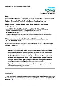
1 Introduction The field of Wireless Sensor Networks (WSNs) has captured the imagination of the world with their potential to enhance human lives. WSN has wide applications in fields like agriculture monitoring, industrial monitoring, smart housing, automobile industry, and in military applications. Wireless sensor network (WSN) consists of a large number of small sensors capable of sensing, processing, and transmitting information to each other. These sensors communicate with other parts of networks using wireless interface.
Figure 1: Wireless Sensor Network. The design of WSNs depends on the environment, the applications objective, cost, hardware, and system constraints such as a limited energy, shortage of communication range and bandwidth, and limited processing and storage in each node. The environment determines the networks factors like size, topology and schemes. There are five types of WSNs: Terrestrial WSN, Underground WSN, Underwater WSN, Multi-media WSN, and Mobile WSN [1]. Terrestrial WSNs: Consist of a number of inexpensive wireless sensor nodes deployed in a given area. Underground WSNs: a number of nodes deployed underground to sense the surrounding conditions. Besides that, sink node is deployed to gather these sensed data to base station. Underwater WSNs: Consist of a number of sensor nodes and vehicles deployed underwater used to monitor underwater conditions. Multi-media WSNs: Consist of a number sensor nodes equipped with cameras and microphones. Used to monitor and track events in the form of video, audio, and imaging. Mobile WSNs: Consist of a collection of sensor nodes that can move on their own. A key difference is mobile nodes have the ability to reposition and organize itself in the network. Large portion of ocean research conducted by placing sensors (that measure current speeds, temperature, salinity, pressure, chemicals, etc.) into the ocean and later physically retrieving them to download and analyze their collected data. This method does not provide real-time analysis of data, which is critical for event prediction. The real-time monitoring of underwater introduces the need of underwater wireless sensor networks. Underwater
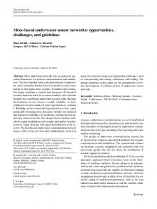
P age |2 wireless sensor network communication has received increased attention motivated by many scientific, military, and commercial interests because it can enable a broad range of applications. The major contribution of this paper is to give an introduction to underwater wireless sensor networks (UWSNs) its characteristic, challenges, applications, and architectures. A comparative study of some existing routing protocols, gives the advantages and limitations of one protocol over the others. Due to resource limitation, it is quite difficult to provide a strong security to UWSNs. This paper identifies the security requirements for UWSN, attacks against UWSNs, and particular solutions for these attacks. Furthermore, a security comparison between the existing routing protocols is given. This comparison clarifies the vulnerability of those routing protocols to various security attacks. Finally, the paper suggests new research directions as a future scope of study in UWSNs. In the rest of this paper, introduction to UWSNs its characteristic, challenges, applications, and architectures introduced in Section 2. Section 3 discusses some existing UWSNs routing protocols and give a comparison between them. In section 4, the security requirements, security attacks, and attacks defenses are presented. Section 5 elaborates the different model and simulation tools are used. Localization methods are outlined in Section 6. The proposed new directions of study are discussed in section 7. Finally, a brief conclusion is given in Section 8. 2 UnderwaterWireless Sensor Network (UWSN) From many decades, there has been a big interest in monitoring the underwater environment for scientific, commercial and military operations. Real time monitoring is very important for many applications, this calls the need of building Underwater Wireless Sensor Networks (UWSNs). UWSNs consist of sensor nodes, surface stations and autonomous underwater vehicles (AUVs) networked to perform collaborative monitoring tasks.
Figure 2: Underwater Wireless Sensor Network. 2.1 UWSNs Challenges The major challenges in the design of UWSNs are [2-4]: Underwater sensors are expensive in terms of equipment, deployment, and maintenance. Network Components: Underwater ordinary nodes, sinks, AUV, and onshore base station. The memory limited by the capacity of the on-board storage device. Battery power is limited and batteries cannot recharge, as solar energy cannot exploit. The available bandwidth is limited depending on the frequency. Acoustic systems operate below 30 kHz. Sensors are prone to failure because of fouling and corrosion and sensors size is large. Dynamic network topology, as nodes tend to be mobile, due to their self-motion capability or random motion of water currents. Routing: Due to high movement of nodes in water current. Range: Usually used in vast ocean areas. Propagation delay in underwater is higher than in Radio Frequency (RF) terrestrial channels by five times. Connectivity loss and High bit error rates (shadow zones). The impaired channel due to multipath and fading. Reliability to guarantee the data is delivered to the surface sink. Time synchronization is difficult to achieve in the underwater scenario due to long propagation delay and variable sound speed and so the localization. Variation in Sound Speed due to temperature, pressure and salinity. Variations in any one of these factors alter the sound speed. It may introduce error in distance estimation and accuracy of the scheme may decrease. 2.2 UWSNs Communication System Underwater communication system involves a transmission of information using any media, either acoustic waves, electromagnetic waves or optical waves [5].
P age |3 Table 1: A comparison between different modes of communication in UWSNs [5].
Acoustic
Electromagnetic
Optical Waves
Speed (m/s)
1500
33,333,333
33,333,333
Bandwidth Range Power Loss
1 KHz 1 km >0.1 dB/m/Hz
1 MHz 10 m 28 dB/1km/100MHz
10-150 MHz 10-100 m depends on turbidity
Electromagnetic Wave: The communication established at higher bandwidth and frequency. However, high absorption /attenuation cause limitation that significantly affects the transmitted signal. Big antennas needed for this type of communication, thus affecting the design complexity and cost. Optical Wave: Offer high data rate transmission. However, absorption and scattering effect influence the signal and the accuracy. Acoustic Wave: The most preferred signal used in many applications, due to its low absorption characteristic in underwater communication. Although the data transmission is slower as compared to other, but the low absorption characteristic enables the signal to travel at longer range as less absorption faced.
2.3 UWSNs Architecture There are three different architectures for UWSNs [6]: 2.3.1 Static Two-Dimensional Underwater Sensor Networks All the nodes anchored to the ocean floor. An uw-sink collects the data from the sensor nodes by the horizontal transceiver. Then, it relays the information to a surface station by the vertical transceiver.
Figure 3: Static two-dimensional UWSN [1]. The surface station has RF signal to communicate with the onshore and surface sinks, as shown in figure 3. The sensors communicated with the sink using direct links or multi-hop paths. In the direct link: each sensor directly sends data to the selected sink. This may not be the most energy efficient. In multi-hop path: the source sensor relayed the data to intermediate sensors until reaches the sink. This saves the energy and increases the network capacity, but also increases the difficulty of the routing. 2.3.2 Static Three-Dimensional Underwater Sensor Networks Each node attached to a buoy by a cable. The sensed data transmitted to the central station by the buoy using RF signal. However, floating buoys may block ships navigating, or can be noticed and turned off by opponents in military applications. The scheme whose sensor nodes anchored to the bottom can overcome this. The sensors anchored to the seabed and fitted out with floating buoys. The buoy pays the sensor towards the water surface as in figure 4. The lengths of the cables are different for the required depth. 2.3.3 Three-Dimensional with Autonomous Underwater Vehicles It consists of lots of static sensors together with some autonomous underwater vehicles (AUVs), as shown in figure 5. AUVs play a key role for additional support in data harvesting. AUVs could considered as super nodes, which have more energy, can move independently, and it could be a router between fixed sensors, or a manager for network reconfiguration, or even a normal sensor. [7] proposes a specialized architecture for UWSNs to provide Energy Efficient and Robust Architecture
P age |4
Figure 4: Static three-dimensional UWSN (Node anchored to the bottom) [1]. 2.4 UWSNs Applications Applications of underwater networks fall into similar classifications as terrestrial sensor networks as follow [8]: Scientific applications: Which observe the environment from geological procedures on the seabed, to water characteristics (temperature, salinity, oxygen levels, bacterial and other pollutant content, dissolved matter) to counting or imaging animal life (micro-organisms, fish or mammals). Industrial applications: Which monitor and control commercial process, such as underwater tools related to oil extraction. Military and homeland security applications: Which include securing and monitoring port facilities or ships in foreign ports, and communicating with submarines. Shallow Water Acoustic Network for Mine Countermeasures Operations. Wireless Sensor Networks on the Great Barrier Reef. UASN for Early Warning Generation of Natural Events. Sensor Network Architectures for Monitoring Underwater Pipelines. Autonomous Underwater Surveillance Sensor Network (AUSSNet). Group-based UWSN for Marine Fish Farms. Underwater Acoustic Network for the Protection of Offshore Platforms and Energy Plants. SeaSTAR Underwater Monitoring Platform.
Figure 5: Static three-dimensional with AUV [1]. 3 Routing Protocols in UWSNs The process of forwarding data from source nodes to a sink is a very challenging task especially in mobile nodes. Saving energy is a major concern. At the same time, node mobility is handled. Routing protocols divided into three categories proactive, reactive and geographical. Proactive or table driven effect a large overhead in order to create the routs, either periodically or every time when the topology modified. Reactive protocols are more appropriate for the dynamic networks, but they cause large delays and require the source to initiate flooding of control packets in order to create the paths. This makes both types of routing protocols unsuitable for UWSNs. Geographic routing considered the promising routing protocol for UWSNs. Geographical routing is a routing principle that relies on geographic position information. The source sends its packets to the geographic location of the destination instead of the destination network address [6]. According to how many nodes host the service four possible combinations can be resulted as some-for-some, some-for-all, all-for-some and all-for-all. It can be classified into three categories: Greedy, Restricted directional flooding and Hierarchical [9-11].
P age |5
a) Greedy:It do not create and maintain paths from source to the destination; as an alternative, a source node includes the approximate position of the receiver in the data packet and selects the next hop according the optimization process of the protocol; the closest neighbour to the destination for example. VBF (Vector Based Forwarding), HH-VBF (Hob by Hop VBF), VBVA (Vector-Based Void Avoidance), ES-VBF (Energy Saving VBF), and CVBF (Clustering VBF Protocol) are some of the popular geographic routing protocols for UWSNs. b) Restricted Directional Flooding: The sender will broadcast the packet to all single hop neighbours towards the destination. The node which receives the packet checks whether it is within the set of nodes that should forward the packet. If yes, it will retransmit the packet. Otherwise the packet will be dropped. In restricted directional flooding, instead of selecting a single node as the next hop, several nodes participate in forwarding the packet in order to increase the probability of finding the shortest path and are robust against the failure of individual nodes and position inaccuracy. The focused beam routing (FBR) Directional flooding routing (DFR) and sector-based routing with destination location prediction (SBR-DLP) are the example for that. c) Hierarchical: Form a hierarchy in order to scale to a large number of mobile nodes. LCAD is an example for that. 3.1 Vector-Based Forwarding Protocol (VBF) VBF is a source routed routing protocol where each packet carries routing information in its header. The idea of a vector like a virtual routing pipe proposed and all the packets forwarded through it. Each packet contains three position fields, SP, TP, and FP, that is, the position of the source, the target, and the forwarder respectively. In addition, each packet contains RANGE field that controls the area where the packet flooded and RADIUS field that defines the radius of the routing pipe [12]. In figure 6, is the source node, and is the sink. The routing ⃗⃗⃗⃗⃗⃗⃗⃗⃗ vector is . Packets forwarded from to . Forwarders forms routing pipes are along the routing vector with a pre-controlled radius (the distance threshold W). Upon receiving a packet, each node calculates its distance to the forwarder and the angle of arrival of the signal. If a node decides that, it is near to the routing vector, it puts its own position in the packet (FP) and forwarding the packet. Otherwise, it discards the packet. The sensor nodes in the pipe are responsible for packet forwarding. Nodes, which are not near to the routing vector, do not forward. Routing in VBF is carried out by query packets in deferent ways:A. Sink Initiated Query There are two types of such queries: Location-dependent query, the sink is interested in a specific area and knows the location of this area. The sink broadcasts an INTEREST query packet, which carries the information of SP and TP. The direction of this query is the targeted area following the pipe defined by SP and TP.
Figure 6: Vector Based Forwarding (VBF) [1].
Location independent query, the sink needs some specific type of data regardless of its location. The sink issues the INTEREST packet carries invalid position for the target. This query will be flooded to the target area. Upon receiving such query, each node checks if it has the data, which the sink needs. If so, the node calculates its position and sends back the data packets needed to the sink. If not, it puts its position in the FP field and forwards the packet.
P age |6 B. Source Initiated Query Sensor node senses some events and wishes to notify the sink, it broadcasts a DATA READY packet. Upon receiving this packet, each node calculates its position and puts its position in the FP field and forwards the packet. When the sink receives such packet, it computes its position. Then it decides if it interests in such data. If so, it sends a location-dependent INTEREST packet to the source. Since the source node is moving, its location computed by the old INTEREST packet might not be true anymore. The source is sending packets to the sink and the sink makes use of the information of the source location carried in the packets to decide if the source is moving out from its interest area. If so, the sink sends the SOURCE_DENY packet to stop this source from sending data. In the other hand, the sink initiates another interesting query to discover a new source. 3.1.1 Self-Adaptation Algorithm All the nodes located within the routing pipe are capable to forward packets. In dense networks, many nodes might be concerned in the data forwarding. In order to save energy, it is necessary to regulate the forwarding based on the node density. It is infeasible to determine the node density due to the mobility. The selfadaptation algorithm allows each node to guess the density in its location and forward packets adaptively. This algorithm based on the definition of a desirableness factor . This factor measures the compatibility of a node to forward the packet.
P is the projection length of node A onto the routing vector⃗⃗⃗⃗⃗⃗⃗⃗⃗ . d is the distance between node A and forwarder F. θ is the angle between vector⃗⃗⃗⃗⃗⃗⃗ and vector ⃗⃗⃗⃗⃗ . R is the transmission range. W is the radius of the routing pipe.
Figure 7: Desirableness Factor [1]. When a node receives a packet, it determines if it is eligible for packet forwarding. If yes, the node waits a time interval then forwards the packets. This time interval based on the node's desirableness factor, a smaller desirableness factor, a less time to wait. √ : A pre-defined maximum delay. : The acoustic signals in water‟s propagation speed, 1500 m/s. : The distance between this node and the forwarder. During the time period if a node receives the same packet from n other nodes, this node should calculate its desirableness factors relative to these nodes, and the original forwarder. If min ( )< where is a predefined initial value of desirableness factor (0≤ ≤3), then this node forwards the packet; if not, it discards the packet.
Figure 8: Self-Adaptation Algorithm [12].
P age |7 In figure 8, the node F is the present forwarder. There are three nodes, A, B, and D in its transmission range. Node A has the minimum desirableness factor. Therefore, A has the lowest delay, it sends the packet first. Node B discards the packet because it is in the transmission range of node A. Node D is not in the transmission range of A. Thus, D also forwards the packet. 3.1.2 Advantages of VBF Reduces network traffic as only the nodes along the forwarding path are concerned in packet forwarding, hence saving the energy of the network. The packet delivery ratio increased in dense networks. 3.1.3 Disadvantages of VBF Sensitivity to the routing pipe‟s radius. Small data delivery ratio in sparse networks. Multiple nodes acting as relay nodes in dense networks. Increase the communication time and energy consumption in dense networks. In case of a void, VBF cannot find a path to forward the packet. 3.2 Hop-by-Hop Vector-Based Forwarding Protocol (HH-VBF) It based on the same idea of routing vector as VBF, the routing virtual pipe redefined to be a per-hop virtual pipe, instead of a single pipe from the source to the sink [13]. As we can see in figure 9, in HH-VBF, nodes A and C can reach the sink by using paths that are not possible with VBF. In HH-VBF the Self-Adaptation Algorithm is different from that in VBF. Each forwarder maintains a selfadaptation timer, which based on the desirableness factor. The timer defines the time the node waits before forwarding the packets. 3.2.1 The Self-Adaptation Algorithm The self-adaption algorithm in HH-VBF is different from that in VBF. In HH-VBF, each forwarder maintains a self-adaptation timer , which depends on the desirableness factor. The timer represents the time the node holds the packet before forwarding it. The desirableness factor of a node A, is defined as
d is the distance between node A and candidate forwarder F. θ is the angle between vector⃗⃗⃗⃗⃗⃗ and vector ⃗⃗⃗⃗⃗ . R is the transmission range.
Figure 9: VBF vs. HH-VBF [1]. The node with the lowest desirableness factor will forward the packet first. In this way, a node may hear the same packet multiple times. The node computes its distances to the different vectors from the packet received to the sink. If the minimum one of these distances is still higher than the pre-defined minimum distance threshold β, this node will send the packet; if not, it discards the packet. The bigger β is the more nodes will forward the packet. Thus, HH-VBF can control forwarding redundancy by adjusting β. 3.2.2 Advantages of HH-VBF: Less sensitive to the routing pipe radius than VBF. The packet delivery ratio increased in dense networks. More paths for data delivery in sparse networks compared to VBF. 3.2.3 Disadvantages of HH-VBF: More packet overhead compared to VBF due to its hop-by-hop nature. Large propagation delay due to its hop-by-hop nature. High energy consumption in dense network. In case of a void, the forwarder is unable to reach any node other than the previous hop. 3.3 Vector-Based Void Avoidance (VBVA) Some areas of the network might not occupy with nodes (Void); VBVA extends the VBF to handle this problem. Initially, the forwarding path of a data packet represented by a routing vector from the source to the destination.
P age |8 If there is no presence of a void, VBVA acts the same as VBF. When there is a void, VBVA uses one of the two mechanisms that have, vector-shift mechanism or back-pressure mechanism, to overcome the void [14]. 3.3.1 Void Detection A node detects the presence of a void by overhearing the transmission of the packet by its neighboring nodes. For forwarding vector⃗⃗⃗⃗⃗ , and a node N, we define the advance of node N as the projection of the vector ⃗⃗⃗⃗⃗ on the forwarding vector⃗⃗⃗⃗⃗ . We call a node a void node if all the advances of its neighbors on the forwarding vector carried in a packet are smaller than its own advance. In figure 10, the advances of nodes B, C and F denoted as . All the neighbors of node F have smaller advances than F. Thus, node F is a void node.
Figure 10: Void Detection [6]. 3.3.2 Vector-Shift Mechanism When a node determines that it is a void node, it will try to bypass the void by shifting the forwarding vector. To do that, the node broadcasts a vector-shift packet to all its neighbors. Upon receiving this control packet, all the nodes outside the current forwarding pipe will try to forward the corresponding data packet following a new forwarding vector from themselves to the target. After shifting the forwarding vector of a packet, a node keeps listening to the channel to check if there is a neighbor node forwards the packet with the new forwarding vector. If the node does not hear that, the packet forwarded even if it shifts the current forwarding vector, the node defined as an end node. For an end node, the vector-shift mechanism cannot find an alternative routing path and it have to use the back-pressure mechanism.
Figure 11: Vector-shift mechanism [1]. In figure 11, the dashed area is a void area. Node S is the sender and node T is the target node. S forwards the packet along the forwarding vector ⃗⃗⃗⃗ then it keeps listening to the channel for some time. Since the neighbor node, D and A of S are not within the forwarding pipe, they will not forward this packet. Node S cannot overhear any transmission of the packet and concludes that it comes across a void. It then broadcasts a vector-shift control packet asking its neighbors to change the current forwarding vector to ⃗⃗⃗⃗⃗ and⃗⃗⃗⃗⃗⃗ nodes D and A repeat the same process. 3.3.3 Back-Pressure Mechanism When a node finds out that it is an end node, it broadcasts a control packet, called Back-Pressure (BP) packet. Upon receiving this control packet, every neighboring node tries to shift the forwarding vector if it has never shifted the forwarding vector of this packet before. Otherwise, the node broadcasts the BP packet again. The BP packet will be routed back in the direction moving away from the target until it reaches a node which can do vector shifting to forward the packet toward the target. In figure 12, the dashed area is a void area. The node S is the sender and node T is the target. When S forwards the packet with forwarding vector ⃗⃗⃗⃗ to node C, since node C cannot forward the packet along the vector ⃗⃗⃗⃗ any more. It will first use vector-shift mechanism to find alternative routes for the data packet. Since node C is an end node, it cannot overhear the transmission of the packet. Node C then broadcasts a BP packet. Upon receiving the BP packet, node B first tries to shift the forwarding vector but fails to find routes for the data packet. Then node B broadcasts BP packet to node A and so on. Finally, a BP packet routed from node A to the source S.
P age |9 Node S then shifts the forwarding vector to ⃗⃗⃗⃗⃗ and⃗⃗⃗⃗ . The data packet forwarded to the target by the vector-shift from nodes D and H.
Figure 12: Back-pressure mechanism [1]. 3.3.4 Advantages of VBVA Solve the void problem. Void avoidance mechanism generates multiple forwarding vectors, which improve the robustness of the network. 3.3.5 Disadvantages of VBVA VBVA void avoidance mechanism introduces more energy consumption. More signalling overhead generated by void avoidance mechanism. Large propagation delay in case of presence of voids. 3.4 Energy Saving VBF Protocol (ES-VBF) ES-VBF introduces node‟s energy information into VBF protocol. The routing process considers both factors of position and energy consumption [15]. VBF algorithm only considers location information to transmit data packet. However, when there is a node whose location is always the best in routing pipe, it will be selected again and again during routing selection. Thus, the energy of this node exhausted, causing routing failure. ES-VBF adds the value of energy consumption into desirableness factor to decide waiting time. Improved desirableness factor : If Node residual energy is larger than 60 % of initial energy:
If the Node residual energy is smaller than 60 % of initial energy: (
)
− : The residual energy of node. − : Initial energy of node. Waiting time is inversely proportional to residual energy. Nodes with higher residual energy have smaller desirableness factor, higher priority of forwarding packets and shorter waiting time among neighboring nodes. 3.4.1 Advantages of ES-VBF Reduces energy consumption of network compared to VBF. Balance the network energy consumption compared to VBF. Prolong the lifetime of network. 3.4.2 Disadvantages of ES-VBF ES-VBF has all the disadvantages of VBF routing protocol. Sensitivity to the routing pipe‟s radius. Cannot handle the void problem. Not suitable in sparse network. Multiple nodes acting as relay nodes in dense networks. 3.5 Clustering Vector-Based Forwarding Protocol (CVBF) The whole network divided into a predefined number of clusters. All nodes assigned to the clusters based on their geographic location. One node at the top of each cluster selected as a virtual sink. The rest of nodes in each cluster transmit the data packets to their respective cluster virtual sink. The routing inside each cluster follows the VBF routing protocol. CVBF defines one virtual routing pipe for each cluster, instead of one virtual routing pipe for all network nodes in VBF. The routing pipe radius is equal to the transmission range of a node. After receiving the data packets from the sensor nodes, cluster virtual sinks perform an aggregation function on the received data, and transmit them towards the main sink using single-hop routing. Cluster virtual sink nodes are responsible for coordinating their cluster members and communicating with the main sink [1, 16]. The algorithm stated in the following steps:
P a g e | 10 3.5.1 Step1: Clustering the Nodes The network divided into groups of nodes according to their geographic location producing non-overlapping clusters excluding the main network sink, which allocated on the water surface. The network space divided into equal space volumes in the form of cuboids as shown in figure 13.
Figure 13: CVBF network area with clusters [1]. The division based on the values of clusters as:
coordinates, and the cluster width
. Choosing the best number of
− : The total surface area of the network − : The area of the cluster surface. The choice of N that gives the value of as near as possible to √ R to make sure that the virtual pipe of the cluster includes all the nodes inside that cluster. 3.5.2 Step2: Selecting the Cluster Virtual Sink For each cluster, which has a space volume × × , choose the node, which is nearest to the main sink to be a cluster virtual sink. If more than one node has the same depth position, we choose the nearest node to the cuboid‟s axis, in which its surface point coordinates is the point ( , , 0). The source node of the cluster is fixed at the position ( , , ). All other nodes can send data to their corresponding virtual sink following the mechanism of VBF and depending on the value of its desirableness factor . ,
.
Figure 14: One cluster and its virtual sink [1]. 3.5.3 Step 3: Calculating the Cluster’s Maintenance Time This step takes into consideration the node mobility that affects network topology and performance. The maintenance algorithm executed simultaneously in all clusters. In this step, a suitable periodical time called maintenance time . Each node in the cluster checks its belonging to that cluster after . If a node belonging to a cluster moves away from that cluster, it naturally has two choices. The first choice is to enter another cluster.
P a g e | 11 The second choice is that it exits from all the network volume. To avoid exiting a node from the network volume, the node positions have to be carefully choosing far from the network space boundaries. − : Maximum distance of a node movement. − : The current speed of the node. 3.5.4 Advantages of CVBF: By studying CVBF protocol, we observe that it has some advantage as: Overcome the pipe sensitive radiuses of VBF. Has high packet delivery ratio compared to VBF. Data delivery ratio in sparse networks is higher than VBF. 3.5.5 Disadvantages of CVBF: We notice that it has some drawbacks as: Virtual sink nodes consume more power when compared to others nodes of the same cluster. Failure of virtual sink nodes will lead to untimely shutdown of its cluster‟s nodes. Cannot handle the void problem. CVBF clustering mechanism causes processing overhead. The protocol handling the node mobility using however, it did not explain a technique that handles the virtual sink mobility “for how long the node act as a virtual sink, and in case of another node closer to the main sink and cuboid‟s axis than the current virtual sink”. No energy balance consumption in the network duo to the asymmetric nodes distribution among clusters. 3.6 Reliable and Energy Balanced Algorithm Routing (REBAR) It is a location based routing protocol that focuses on three significant problems to deal in UWSNs: energy consumption, delivery ratio and handling void problem. First, REBAR uses a sphere energy depletion model to analyze the energy consumption of nodes in UWSNs Then this model is extended by considering the node mobility in UWSNs and they assumed that node mobility is a positive factor which can help balance the energy depletion in the network and prolong lifetime of networks. Each node is assigned a unique ID and fixed range REBAR is based on the following assumptions. • Every node knows its location and of the destination through multi-hop routing. • Sensed data are sent to the destination at a specific rate. 3.7 The Focused Beam Routing (FBR) It assumes that each node knows only its own location and the final destination location. In the proposed protocol, variable transmission power levels are used in the forwarding of data packet, and this transmission power have a range from P1 to P n For each power level there is a corresponding transmission radius d n which is a cone of angle emanating from the source node to the destination, are intended to avoid unnecessary flooding of broadcast queries. It is suitable for networks containing both static and mobile nodes, which are not necessarily synchronized to a global clock. A source node must be aware of its own location and the location of its final destination, but not those of other nodes. 3.8 Directional Flooding Routing (DFR) It focuses on high mobility of nodes and the conditions of aquatic environment and takes into account the link quality in the forwarding strategy. The proposed approach, assumed that the geographic information is available; all nodes know their location, their one-hop neighbors‟ location and the location of a sink. In addition, the nodes are also able to measure the quality of the links with neighbors. DFR also addresses a well-known void problem by allowing at least one node to participate in forwarding a packet. In DFR, a packet transmission uses a scoped flooding, i.e. a flooding zone is created to limit the flooding in the whole networks. This flooding zone is determined using an angle between and, where F is the node which receives a packet, S and D are the source and destination, respectively. 3.9 Location Aware Source Routing (LASR) In this protocol two techniques are adopted for handling high latency of acoustic channels, namely link quality metric and location awareness. All the network information including routes and topology information are passed on in the protocol header. Resultantly header size increases as the hop count between source and sink increases. 3.10 A Sector-Based Routing with Destination Location Prediction (SBR-DLP) It supposes that a node knows its own location, and the location of the destination node is predicted. Consequently, it relaxes the need for accurate knowledge of the destination‟s location. In SBR-DLP the sensor nodes are not required to carry neighbor information or network topology. Each node is assumed to know its own position, and the destination node‟s pre-planned movements. This movement is usually predefined prior to launching the network. The sender decides which will be its next hop using information from the candidate
P a g e | 12 nodes trying to eliminate the problem of having multiple nodes acting as relay nodes. It makes no assumption about the location of the destination node being fixed and accurately known to the sender node. It takes into consideration the entire communication circle to locate the candidate relay node. RTS does not need to be rebroadcasted every time. 3.11 LCAD A clustering algorithm based on the geographical location of the sensor nodes in 3-D Hierarchical network architecture called LCAD. In this protocol, the entire network is divided into 3-D grids. The optimal horizontal transmission range is less than 50m and the vertical transmission range is around 500m; the size of each grid is set approximately to 30m x 40m x 500m. A grid comprises of a single cluster. The data communication is composed of three phases: (i) set-up phase, where the cluster head is selected. (ii) Data gathering phase, where data is sent by the nodes in the cluster to the cluster head. (iii) Transmission phase, where the data gathered by the cluster heads is transmitted to the base station. The selection of the cluster head is based on the sleep wake pattern along with residual memory and energy of the contending Ch-nodes. 3.12 Information Carrying Routing Protocol (ICRP) ICRP makes use of control packets that are carried by data packets. ICRP does not incorporate the use of state or location information, and also only a small fraction of the nodes participate in the routing process. The ICRP incorporates three steps that are, route finding, route preservation and route renunciation. 3.13 Depth Based Routing Protocol (DBR) DBR needs just the depth information of sensor nodes. DBR is a desirous algorithm that tries to direct a packet from a source node to sinks to acquire the depth of current node; each sensor node is outfitted with a reasonable depth sensor. DBR utilizes the various sink construction modeling as a part of which different number of sinks are put on the water level and are utilized to gather the information packets delivered by the sensor nodes. DBR takes the routing decision on the basis of depth data, and advances the information packets from higher depth nodes to lower depth sensor nodes. 3.14 Hop- by- Hop Dynamic Address based Routing Protocol (H2H-DAB) Sensor nodes utilize the dynamic address to get new delivers as indicated by their new positions at distinctive depth levels. This convention utilizes numerous surface buoys that are utilized to gather information and a few nodes are secured at bottom and the rest of the nodes are tied down at diverse depths. Nodes closer to the surface have smaller value of addresses, and these addresses get to be bigger as the nodes travel towards the bottom. In first stage, it assigns the dynamic addresses to the sensor nodes, and in second stage, information is sent utilizing these addresses. With the assistance of hello packets, dynamic addresses are assigned to nodes and these addresses are produced by the surface sinks. 3.15 Constraint Based Depth Based Routing Protocol (CDBR) The sensor nodes are sent under the water haphazardly. Various sinks are sent on the sea level whereas the sensor nodes are in charge of conveying the sensed information to the sinks. RF modems and Acoustic modems are the major parts of the sinks. The sensor nodes under the water are furnished with Acoustic modems. The nodes correspond with one another and the Sinks utilizing the Acoustic Modems. The sinks correspond with one another and the on-shore server farm utilizing the RF Modems. Information arriving at any of the sinks is considered as information conveyed effectively. 3.16 Mobile Delay-Tolerant Approach (DDD) It uses collector nodes called dolphins to gather information that is sensed by the sensor nodes. The recommended scheme shuns multi-hop communication, and data is sent to acoustic nodes that are in its communication range. The sensors occasionally wakeup to sense data and to generate some events. The acoustic modem is centered on two parts. The first part is utilized for acoustic communication with the close dolphin, and the other part is a low-power transceiver used to determine the occurrence of dolphin nodes and the activation of the first component is done through this. 3.17 Performance Comparison of UWSNs Routing Protocols Design a routing protocol is a challenging task. All the nodes inside UWSN should be reachable (Connectivity) while covering process (Coverage), even when the nodes inside the network start to fail due to energy issues or other problems (Fault Tolerance). The protocol should also adapt network size and density (Scalability) and provide a certain QoS. In parallel way, designers must try to use the memory and energy consumption of the protocol efficiently. We compare between all the surveyed routing protocols according to our studies and other related works [17]. Factors such as the amount of deployed nodes in the network regulate metrics dealing with matters of data pack delivery, end-to-end delay and energy consumption. Thus, we compare between these protocols with respect to
P a g e | 13 spares and dense networks. Table 2 summarizes the comparison results for VBF‟s protocol. Table 3 elaborates the comparison between protocols in point of view of their characteristics. Performance comparison is mentioned in Table 4. Table 5 monitors the metrics of protocols where Table 6 discusses the application and advantage and disadvantage of each protocol. Table 2: Comparison among VBF routing protocols [ ]. VBF
HH-VBF
VBVA
ES- VBF
Handle void Suitable to Be Implemented in
CVBF
Cluster Head Dense
Sparse
Mobile Nodes Static Nodes
Dense
High
High VBF
Sparse
Low
More robust than VBF
Low as VBF
Single/Multi Sink
Single
Single
Single
Single
Forwarder node criteria
Distance
Distance
Distance
Distance/ energy
Distance
Sinks deployment
One fix on surface
One fix on surface
One fix on surface
One fix on surface
Multi virtual /one fix on surface
ForwardingShape Region
Single pipe routing
Per-hop pipe routing
Single pipe routing / Multiple pipe routing in case of void presences
Single pipe routing
Single routing cluster
Sensitivity to routing pipe radius.
High sensitive
Less sensitive than VBF
Not sensitive
High sensitive as VBF
Not sensitive
Dense
High
High
High
High
High
Sparse
Low
Low
High
Sparse
Low
Higher than VBF & HH-VBF High as High in VBF void Low as presences VBF
Low
Dense
Dense
Low
Sparse
High
Higher than VBF Higher than VBF Higher than VBF Higher than VBF Less than VBF
Network design
Robustness
Data Delivery Ratio Energy Consumption
End to Delay
End
as
High as VBF
More robust than VBF & HH-VBF in void presences
Low as VBF Less than VBF & HH-VBF
High VBF
as
Low VBF
as
Less than VBF Low as VBF Higher than VBF High as VBF
High as VBF
Low in case of Low virtual as sink VBF failure Single virtual sink per cluster
pipe per
High as VBF Low as VBF Low High as VBF
4 Security in UWSNs UWSNs used in various fields of interest with increasing need for security. This need for security appeared in case of military applications or applications working with sensitive data. Compared to the research in security for WSNs, UWSN security research is limited. Achieving security objectives in UWSNs is a challenging task due to the special constraints of underwater environment. Nodes have limited processing capability, very low storage capacity, limited bandwidth, and limited energy. Therefore, security services in UWSN should protect the information over the network and take into account the limited resources of the nodes. 4.1 Security Requirements In order to achieve security in UWSNs, security requirements should be provided [3, 5, 18]. These security requirements represented in Table 7. 4.2 Security Threats UWSNs are susceptible to security attacks because of the broadcast nature of the transmission medium. Moreover, UWSNs have an additional vulnerability because nodes not physically protected. Attackers may do
P a g e | 14 various types of security threats to make the UWSN system unstable [18]. A useful means of classifying security attacks is in terms of passive attacks and active attacks. 4.2.1 Passive Attacks The goal of the adversary is to obtain the information that is being transmitted. No alteration of data makes passive attack difficult to detect. Passive attacks are also known as Attacks against Privacy. There are some common attacks against privacy are: Monitor and Eavesdropping: an adversary could eavesdrop and intercept transmitted data. To prevent these problems we should use strong encryption techniques. Traffic analysis attacks: the attacker predict the nature of communication by captures the packets in order to analyze the traffic, determines the location, identifies communicating hosts, and observes the exchange of the message. Using all these information, they predict the nature of communication. 4.2.2 Active Attacks It involves modification or creation of a false packet. The adversary able to control all the data sent. There are some common active attacks are: Modification: The adversary can simply intercept and modify the packets‟ content. Replay: The adversary re-transmits the contents of the packets later. Injection: the attacker sends out false data into the network. An attacker compromises the sensor by different ways, gains control or access to the sensor node itself. Attackers can physically breaking into the hardware by modifying its hardware structure, or by taking the data from the hardware device without any form of hardware structural modification. The compromised node then behaves in some malicious ways, e.g., to generate a fake message and to attack the network. Complex attacks from compromised nodes can target the internal protocols used in the network, such as routing protocols. Vulnerability of routing protocols is usually caused by missing authentication, freshness and integrity check of the routing information. This fact is denoted in the following attacks: 4.2.2.1 Sinkhole Attack The goal of this attack is to attract as much of the traffic as possible to the malicious node. The adversary places malicious node to the closest sink. The malicious node tries to look very attractive for other nodes with respect to the routing algorithm. The result is that the neighbor nodes choose the compromised node as the next-hop node to route their data through. Authentication of nodes exchanging routing information or redundant paths can defense this attack. 4.2.2.2 Selective Forwarding Attack An attacker may create malicious nodes which selectively forward only certain messages and simply drop others. In UWSNs it should be confirmed that the receiver is not receiving the information due to the attack and not because it located in a shadow zone. Multi-path routing can effectively defense these attacks However, multipath routing increases communication overhead. Another solution of this attack is to check the sequence number of the data packet.
Figure 15: Sinkhole attack in UWSNs.
P a g e | 15
Table 3: Comparison of routing protocols based on their characteristics [19]. Protocol/ architecture
Single/ Multiple copies
Hop-byhop/ endto-end
Clustered/ single entity
Single/multisink
Hello or control packets
Requirements and assumptions
Knowledge required/ maintained
VBF
Multiple
End-to-end
Single-entity
Single-sink
No
Geo. location is available
Whole network
HH-VBF
Multiple
Hop-by-hop
Single-entity
Single-sink
No
Geo. location is available
Whole network
FBR
Single-copy
Hop-by-hop
Single-entity
Multi-sink
Yes
DFR
Multiple
Hop-by-hop
Single-entity
Single-sink
No
REBAR
Single-copy
Hop-by-hop
Single-entity
Single-sink
No
SBR-DLP
Single-copy
Hop-by-hop
Single-entity
Single-sink
DDD
Single-copy
Single hop
n/a
DBR
Multiple
Hop-by-hop
H2-DAB
Single-copy
LCAD LASR
Geo. location is available Own, 1-hop neighbors and sink info Own, 1-hop neighbors and sink info
Own and sink location
Yes
Geo. location is available
Own location and sink movement
n/a
Yes
Network with special setup
Single-entity
Multi-sink
No
Nodes with Special H/W
About dolphin node presence No network information maintained
Hop-by-hop
Single-entity
Multi-sink
Yes
n/a
1-hop neighbor‟s
Single-copy
Hop-by-hop
Clustered
Single-sink
Yes
Nodes with special H/W
Own cluster information
Single-copy
End-to-end
Single-entity
Single-sink
Yes
Network with special setup
Source to sink information
Own and sink location Own and sink location info.
Remarks Considered as first geographic routing approach for UWSN Enhanced version robustness improved by introducing hop-by-hop approach instead of endto-end A cross layer location-based approach, coupling the routing, MAC and phy. layers. A controlled packet flooding technique, which depends on the link quality, while it assumed that, all nodes can measure it use adaptive scheme by defining propagation range. Water movements are viewed positively does not assumes that destination is fixed plus it consider entire communication circle instead of single transmitting cone A sleep and wake-up scheme, which requires only one-hop transmission Considered 1st depth based routing. After receiving data packet, nodes with lower depth will accept and remaining discards Short dynamic addresses called Hop-IDs are used for routing, assigned to every node according to their depth positions Clusters are formed, in order to avoid multi- hop communication A DSR modification. Location and link quality awareness is included. Preferred only for small networks
P a g e | 16
Table 4: Performance comparison of UWSN protocols [19]. Protocol / architecture VBF HH-VBF FBR DFR REBAR DDD DBR H2-DAB LCAD LASR
Delivery ratio Low Fair Fair Fair Fair Low High High Fair Fair
Delay efficiency Low Fair High Fair Low Low High Fair Low Low
Energy efficiency Fair Low High Low High High Low Fair Fair Fair
Bandwidth efficiency Fair Fair Fair Fair Fair Fair Fair Fair Fair Fair
Cost efficiency n/a n/a n/a n/a n/a Low Fair High Low High
Reliability Low High Fair High Fair Fair High Fair Low Fair
Performance Low Fair High Fair Fair Low High Fair Low Fair
Table 5: Metric comparison of UWSN protocols [9].
Parameter And Protocol
Localization of nodes required
Multi- sink architecture
Technique used
ICRP
No
No
Broadcasting
DFR
Yes
No
Packet flooding
Yes
Broadcasting
Yes
Broadcasting
DBR CDBR
Only depth information Only depth information
Dynamic addressing Virtual routing pipe
H2- DAB
No
Yes
VBF
Yes
No
SBR-DLP
Yes
No
Multicasting
DDD
No
Yes
LASR
Yes
No
Broadcasting Link quality metric and location awareness
Basic parameter onto which routing decision is made Path life- time Base angle or criterion angle Depth of neighbor Depth threshold value Dynamic address Node nearer to the virtual pipe Distance to destination node N/A Shortest path metric
Network topology
Control packets
Routing table required
Dynamic
Yes
Yes
Dynamic
No
Yes
Static
No
Yes
Static
No
Yes
Dynamic
Yes
No
Dynamic
No
Yes
Static
No
Yes
Static
Yes
No
Local
No
Yes
Table 6: Comparison of routing protocols in UWSN [20] . Routing protocol VBF HH-VBF FBR REBAR SBR-DLP DFR LASR
Category
Application
Advantages
Disadvantages
Location based routing
Energy-efficient UASN
a) Energy efficient b) Robustness c) High success of data delivery
DBR
Depth based routing
Dense network application
a) Very high packet delivery ratio b) No need of full dimensional location information of nodes
a) Not energy efficient b) Batteries are stranger to recharge
LCAD
Cluster based routing
Energy-efficient UWSN
a) High scalability and robustness b) Less load and energy consumption
a) Processing overhead is complex
a) Low bandwidth b) High latency c) Delay efficiency, ,performance and reliability are low
P a g e | 17 Table 7: The security requirement of UWSNs [3, 5, 18]. Security Requirement Authentication Confidentiality
Definition
Verifying that communicating nodes are who they claim to be. It can be achieved by Massage Authentication Code (MAC) Hiding the data from everyone except for those who are authorized. It can be achieved by the use of encryption.
Integrity
Ensures that the packet is not altered during transmission.
Availability
Guarantee to provide the network services even when the system is attacked.
Non-repudiation
Prevents the source to deny that it sent that packet.
Freshness
Secure Localization
Self-Organization
To ensure that the data is recent, and to ensure that no old messages can be replayed. The ability to accurately, and automatically locate each sensor. Localization can help in making routing decisions, so the attackers are searching the header of packet. The secure localization is an important factor during implementing security in the network. It can be achieved by encrypting the header of the packet. Distributed sensor networks must self-organize to support multi-hop routing. Such self-organization is hard to be done in a secure way.
Secure Time Synchronization
Time synchronization is very important for many operations, such as coordinated sensing tasks, and sensor scheduling (sleep and wakeup).
Robustness and Survivability
The sensor network should be robust against various security attacks, and if an attack targets, then its impact should be minimized.
Figure 16: Selective Forwarding attack in UWSNs. 4.2.2.3 Sybil attack An advanced version of an impersonate attack, in which an attacker can forge identities of nodes by appearing in multiple places at the same time. Geographical routing protocols are also vulnerable because an adversary with several identities can claim to be in multiple locations at once. Authentication and position verification are methods to protect against this attack, while position verification is difficult in UWSNs due to the mobility. 4.2.2.4 Homing Attack Some nodes may have special responsibilities, such as sink node and cluster-head node. These nodes attract malicious attacker‟s interest. He tries to block the normal function of these nodes. Once these nodes failed or compromised, the whole or a portion of the network might become useless. Location based forwarding protocols expose to such attack. The attacker passively listens to the network and learns the location of such nodes. Then these nodes are attacked and brought down. One approach is to encrypt the packets headers to hide the location of the important nodes. 4.2.2.5 Wormholes Attack Two malicious nodes cooperate by tunneling packets to establish shortcut appearance using private communication channel which lead to increase the probability of being selected path. Then, it drop packet and analysis traffic. Routing protocols choose the paths that hold wormhole links because they seem to be shorter. Location based protocols can also be vulnerable to this attack when malicious nodes claim wrong locations and mislead other nodes. A general solution for detecting and countering wormhole attacks based on packet leashes. Two types of packet leashes introduced namely temporal and geographical leashes.
P a g e | 18
Figure 17: Sybil attack in UWSNs. 4.2.2.6 Jamming Attack An adversary injects unwanted signals into the communication channels. These signals can occupy the communication channel such that legitimate communication cannot take place or corrupt the packets in transmission. Most common defense against jamming attacks is to use spread spectrum techniques and switching nodes to a lower duty cycle hence, preserving power.
Figure 18: Wormholes attack in UWSNs. 4.2.2.7 Tampering An attacker can damage or modify nodes physically. Due to underwater nodes may be deployed in enemy zone and the network may consist of hundreds of nodes spread large scales, we cannot ensure the safety of all nodes. An attacker may compromise nodes to read or modify its internal memory. Traditional physical defenses include hiding nodes. 4.2.2.8 Acknowledgment Spoofing A malicious node overhearing packets sent to its neighbor nodes used to deceive link layer acknowledgments with the objective of reinforcing a weak link which is located in a shadow zone. Shadow zone is a distributed routing protocol and these are formed when the acoustic rays are bent and sound waves cannot pass into the network which can cause high bit error rates and loss of connectivity in the network. Counter measure are: Encryption of all packets sent through the network. 4.2.2.9 Hello Flood Attack A malicious node send a hello packet that may interpret the false assumption about the attacker is a neighbor and the node will assume that the neighbor node is inside the radio range and forward all the packets to the malicious node. The transmission power is very high for adversary node when compared with the other nodes in the network. Bidirectional link verification method can protect against this attack, although it is not accurate due to mobility of the nodes and the high propagation delays of UWSNs. Authentication is also a possible defense. It can be overcome using following two techniques are: 1. Bidirectional link verification. 2. Authentication in a possible defense. 4.2.3 Security Comparison UWSN security is a critical issue to consider when designing network system. Due to data theft, data changes, energy and cost consuming, a secure environment to rout data becomes one of the essential needs. However, the
P a g e | 19 surveyed routing protocols designed without the consideration of security issues. A comparison of different attacks on the surveyed routing protocols of UWSN based on their nature and goals is given in Table 8. Table 8: Security analysis among routing protocols [3]. Threats
Condition
Reason
Selective Forwarding
All protocols are secure against it.
Because, all packets exchanged based on flooding technique. However, in case of sparse network and void nodes, all protocols are vulnerable except VBVA.
Sybil Attack
All protocols are vulnerable to it.
Because, there is no authentication mechanism uses by nodes and there is no guarantee that a node is in fact at the position it is claiming.
All protocols are secure against it except CVBF. All protocols are secure against it except CVBF All protocols are vulnerable to it.
Because, all packets exchanged based on flooding technique. However, CVBF would be vulnerable to it, in case of the malicious node placed close to the virtual sink node.
Sinkhole Attack
Homing Attack Eavesdropping Jamming
All protocols are vulnerable to it.
Tampering Attacks
All protocols are vulnerable to it.
Because, there is no special-purpose nodes except in CVBF i.e. Virtual Sink node. Because all packets broadcasted without using any encryption mechanism. Because all packets broadcasted in a shared communication channel. Thus, an adversary can inject unwanted signals into this communication channel. Because the deployment of the nodes is on an open /dynamic /hostile environment thus, physical access, capture and node destruction could be done.
The surveyed protocols are Location-based routing protocols and they based on the broadcast nature of the acoustic channel which make them vulnerable to security attacks, given that packet information can be overheard by passive intruders or unauthorized nodes. In other hand, this Location-based technique increases the concerns of securing the location information, which included in each data packet transmitted. Moreover, since no governing mechanism exists to verify that a node is in fact at the position it is claiming, malicious attackers can easily exploit the system. Furthermore, the holding time, used to schedule the forwarding of data packets, allows malicious attacker to exploit these protocols and implement various routing disruptions on the network. Table 9 summarizes all the surveyed security attacks, including the attack name, a brief description, and possible solutions. Table 9: Brief description of security attacks and its countermeasures [3]. Attack Sinkhole Selective Forwarding Sybil
Homing attack
Wormhole
Jamming
Tampering
Description The adversary places malicious node to the closest sink. The malicious node tries to look very attractive for other nodes. Inducing the nodes to route the traffic through a set of compromised nodes, which then drop the routed packets. Malicious node impersonates some nonexistent nodes; it will appear as several malicious nodes with multiple identities. An attacker achieves DoS against the special purpose nodes. Once these nodes failed the whole network become useless. Two malicious nodes directly connected, receive packets at one node and tunnels them to the other node. This creates a man in the middle attack and dropping the packets. The jammer determines the frequency of communication then injects unwanted signals into the communication channels. An attacker tries to damage or modify the nodes physically.
Countermeasure Multipath and authentication of nodes exchanging routing information. Supporting multipath and authentication of nodes exchanging routing information. Authentication and position verification. Hiding and Encryption.
Packet leashes. Spread spectrum, lower duty cycle, and mapping the jammed area in the network and routing around it. Traditional physical defenses include hiding nodes.
5 Simulation and Modeling Tools 5.1 Simulation Tools In the underwater sensor network, the acoustic signals are used for communication among nodes because the radio signal works with additional low frequency and it cannot travel far away in underwater. Simulation-based
P a g e | 20 testing can facilitate to signify whether or not the time and monetary investments are valuable. Simulation is the most common approach for testing new protocol. A Number of advantages are like lower cost, ease of implementation, and realism of testing large-scale networks. Table 10 summarizes the simulation programs and its characteristic. Simulation is not as perfect as real environment. Thus, the designs of various simulators created are accurate and most useful for different situations/applications. The tool, which is using hardware as well as firmware to perform the simulation, is called an emulator. Emulation can unite both software and hardware implementation. Typically emulator has greater scalability, which can emulate several sensor nodes at the same time [21]. A) NS-2 NS-2 was designed by Defense Advanced Research Projects Agency (DARPA) and National Science Foundation. Can be used in both wired and wireless networks. NS-2 is an open source tool. Two languages can be used to increase the level of learning a curve. Tool Command Language (TcL) is most probably used for writing simulation code and also gives an absolute learning curve. NS-2 gives some further features of modeling sensor networks of sensor channel models, power models, scenario generation Merits: 1. NS-2 supports a significant range of protocols in various layers. 2. Low cost 3. Users can easily edit the on-line documents and develop their own codes. Demerits: 1. Tool command language is tedious to understand and write 2. NS-2 is more complicated 3. Time consuming for developing a protocol 4. NS-2 does not support GUI. B) EmStar EmStar is an Emulator particularly planned for WSN assembled in C and it was developed by university of California, Los Angeles. EmStar contains both of the simulation and emulation tools, which use a modulator, but with severely layered architecture. EmStar gives a range of services that are used and joint to provide network functionality for wireless embedded systems Merits: 1. Robustness 2. Easy to evaluate faults and error 3. More flexible 4. The master used to decrease bugs Demerits: 1. Limited scalability 2. Decrease reality of simulation 3. The master can be accessed with only real time simulation C) GloMoSim Global mobile Information System Simulator (GLoMoSim) is a scalable simulation for huge wireless and wired Networks. GLoMoSim can run using a numerous of synchronizing protocols, and was effectively implemented on equally shared memory and distributed memory computers. GLoMoSim provide fundamental functionality to stimulate wireless networks. Merits: 1. Large scalability 2. It supports adhoc networking protocols 3. Good mobility models Demerits: 1. GloMoSim supports only wireless network 2. Effectively limited to, IP networks 3. No specific routing protocols 4. Difficult to stimulate large sensor networks. D) Shawn Shawn is an open source and also a customizable sensor network simulator. Shawn (simulation/programming language) can be written in Java. It consists of features perseverance and decoupling of the simulation surrounding. They decouple state variables that allow for an easy implementation of persistence. In Shawn, two nodes can be easily communicated with exchanging messages that can be identified with communication models. Merits: 1. Dense Protocol can be replaced by modifying 2. Easy to determine the effect of channel Parameters.
P a g e | 21 Demerits: 1. Simulation issues or lower layer issues are not considered. 2. Limited to generate a postscript file. E) UWSim UWSim is primarily designed for Underwater Sensor Network. UWSim is mainly focusing on some specific handling scenarios like low-bandwidth, low frequency, high transmission and limited memory. It is based on component-based approaches slightly than a layer/protocol-based approach. Basically UWSim is based on a novel Routing protocol which is proposed by Developers, distinct traditional simulators which are based on moreover Proactive or reactive routing protocols (AODV and DSR). Demerits: 1. Restrict the number of functionalities. 2. It cannot be used for any other sensor network of UWSN. F) VisualSense VisualSense is planned to maintain a component-based structure of such models. VisualSense offers an exact and extensible radio model Demerits: 1. It will provide a protocol only to the sound. G) JSim J-Sim based on the concept of autonomous component architecture (ACA). J-Sim consists of three level components which are targeted nodes, the sensor node, sink node. JSim gives GUI library. J-Sim also offers a script interface that allows integration with various script languages such as Perl, Tcl or Python. Merits: 1. High quality of reusability and interchangeability 2. Independent platform 3. Lots of memory space. Demerits: 1. Difficult to use 2. Execution time is high 3. Makes user hardly to use H) OMNeT++ Is an Object-oriented distinct network simulation framework. OMNeT++ is not a simulator, but it slightly gives a framework and tools to write simulations Merits: 1. Provide a powerful GUI. 2. Much easier simulator 3. Simulate power consumption problems in WSN 4. A Simulator can support MAC protocol as well as some localized protocol in WSN. Demerits: 1. Available protocols are not large enough 2. Compatible problem will arise 3. High probability reports bugs I) Aqua-Sim Aqua-Sim can efficiently simulate the acoustic signal attenuation and packet collisions within underwater sensor networks. Aqua-Sim can easily be included with the accessible codes in NS-2. Aqua-Sim is equivalent with the CMU wireless simulation packages. Aqua-Sim which is not affected by any alters in the wireless package and it is independent of the wireless package]. Further, any modification to Aqua-Sim also limited to itself and does not have any collision on other packages in NS-2. Aqua-Sim can be designed with extensible and flexible options. It consists of three basic classes like Entities, Interfaces and Functions [22]. Merits: 1. Discrete-event driven network simulator 2. 3D networks besides mobile networks are supported. 3. High fidelity simulation for underwater acoustic channels. 4. Easily import new protocols Demerits: 1. In underwater, acoustic signals are very slow. J) QualNet QualNet is a planning, testing and training tool that “mimics” the activities of an actual communication network. QualNet gives a complete environment for design Protocol, creating and animating network scenarios. QualNet
P a g e | 22 consists of graphical tools that show more numbers of metrics gathered during simulation of network scenario. QualNet can maintain real-time speed to allow software-in-the-loop. QualNet can execute on a cluster, multicore and multi- processor systems. Merits: 1. High speed 2. It can model, thousands of nodes 3. Scalability 4. Extensibility.
Simulator NS-2 EmStar GloMoSim Shawn UWSim VisualSense J-Sim OMNeT++ Aqua-Sim QualNet
Table 10: Comparison of UWSN simulation programs [21]. Open Source and Programming Online Limitations Language/Platform Documents C++ Yes Complicated, Time consuming GUI didn't support. Limited scalability, Decrease reality of simulation, Linux Yes Accessed by only a real time simulation Currently supports only wireless network, Parsec Yes Effectively limited to IP networks, No specific routing protocols Low layer issues are not considered, Limited to Java Yes generate postscript files. Restricted number of functionalities, Not usable for C++ any sensor networks except UWSN. Ptolemy II Provides a protocol only to the sound signal. Java Yes Difficult to use, Execution time is high. Noncommercial License, Compatible problem, High probability of bug C++ Commercial report. License C++ Yes An acoustic signal is very slow Commercial C++ License
5.2 Modeling Tools Modeling is a representation of a system that allows for investigation of the properties of the system and, in some cases, prediction of future outcomes. The main motivation behind building a model is to correct design errors and other shortcomings before the construction of the real building starts. Coloured Petri Nets [23] (CPnets or CPNs) is a graphical language for constructing models of systems and analyzing their properties. CP-nets is a modeling language combining the capabilities of Petri nets with the capabilities of a high-level programming language. An advantage to using CPNs is to use the same models to check both the logical or functional correctness of a system. 6 Localization There are many techniques available for localization in Wireless Sensor Network (WSN) but they are not applicable in UWSN. GPS signals cannot be used underwater for localization. Underwater communication is based on acoustic waves. These localization methods are divided into two approaches: Range-based schemes and Range-free schemes [4]. a) Range-Based Localization Schemes Range-based localization schemes use range or bearing information for position estimation. These may use Time of Arrival (TOA), Time Difference of Arrival (TDOA) or Received Signal Strength Indicator (RSSI) for distance estimation. Location of some nodes in network is known in advance which are called anchor node or reference node. These are used to localize other non-localized nodes in the network. First of all, distance is measured between sensor node and some anchor nodes. Then these distance measurements are used to find node‟s position coordinates. An Anchor Free Localization Algorithm (AFLA) is scheme, where no anchor nodes are deployed. Sensor nodes are connected to fix anchors by cable at sea bottom to avoid them to move away from monitoring area. It is selflocalization algorithm that makes use of relationship of adjacent nodes for position estimation. A Hierarchical Localization Approach (LSL) for large-scale 3D network is scheme where for ordinary node localization, a distributed approach is used that integrated 3D Euclidean distance estimation with recursive
P a g e | 23 location estimation method. There are three types of nodes: surface buoy, anchor node and ordinary node. Surface buoys get their location through GPS and helps in anchor nodes localization. Anchor nodes in turn are used to localize ordinary nodes. High localization coverage with low communication overhead can be achieved by this scheme. A Time Synchronization Free Localization Scheme (LSLS) for large scale UWSN. Three surface buoys are deployed that can hear each other. It relies on time difference of arrival measured at a sensor node from three anchor nodes that can hear each other. Reactive beaconing is used for time synchronization. An iterative procedure is followed in which localized nodes become reference nodes in next round to maximize coverage. Effect of variable sound speed on the scheme is evaluated. High node density is required for large area coverage. A distributed bilateration projection based method for 3D UWSN called Underwater Sensor Positioning (USP). 3D localization problem is transformed to its 2D counterpart by employing depth information of sensor nodes Bilateration and iterative localization is used to localize all nodes in 3D network with the help of three surface buoys. A node is localizable in 2D plane if it is localizable in 3D plane. Bilateration can localize more nodes than can be localized by trilateration. Underwater Positioning System (UPS) scheme: It is a silent positioning scheme that does not require time synchronization among nodes. Four reference nodes including one deployed underwater are used. Time difference of arrival from reference nodes is used for range measurement by sensor nodes. An extended version of UPS called Wide Coverage Positioning Scheme (WPS). Five reference nodes are used in WPS to avoid the problem of infeasible region in UPS. Performance of WPS is worsted than UPS but it achieves unique localization with high probability. Dive and Rise (DNR): is used which learn their coordinates using GPS when floating on sea surface and then dive in sea to a certain depth and rise again. During this, message containing their location and time are broadcasted to the sensor nodes. Sensor nodes passively listen to DNR message beacons and calculate their location after getting three or more messages. It is a silent positioning scheme and uses TOA for distance measurement. Multistage localization using mobile beacon (PL) Here DNR scheme is integrated with iterative localization. DNR beacons dive only to a small depth rather than to cover whole monitoring area in this scheme. A node localized by mobile beacons becomes new anchor node and helps to localize other nodes if it lies below maximum dive depth of mobile beacons. Meandering Current Mobility (MCM) model is used to consider node mobility. A Three Dimensional Underwater Localization (3DUL) Localization process is divided into two phases: 1. ranging and 2. Projection and dynamic trilateration. During ranging, estimated sound speed and two ways message are used for distance measurement between sensor node and three neighboring anchor nodes. During 2nd phase, three anchor nodes are projected to plane of to be localizing node. If virtual anchor plane is robust, then trilateration is used to find location.
b) Range-Free Localization Schemes Range free schemes do not deploy range or bearing information i.e. TOA, TDOA, RSSI is not used for localization in these schemes. These are simple techniques and provide coarse-grained location estimation for underwater nodes. An Area Localization Scheme (ALS) estimates node‟s location in a certain area rather than exact location. Each reference node sends acoustic signals at different power level. So area is divided in smaller region based on different power level of reference nodes. Spherical propagation model is used for acoustic signals. Sensor nodes record the minimum power level received for each reference node and send this information to a central server. Central server find the region in which sensor node reside based on that information. Main limitations of this scheme are: 1.It is centralized. 2. Coverage is determined by communication range of reference nodes and 3. It does not provide exact position coordinates A localization scheme Using Directional Beacons (UDB). An AUV with directional antenna moves over a predefined route and sends directional signals at some angle toward sensor nodes Sensor nodes passively listen these signals and localize themselves. It is an energy efficient technique because sensor nodes are only receiving the mobile beacons. Time synchronization among nodes is not required. UDB is extended to 3D underwater network by Localization with Directional Beacon (LDB). LDB is a distributed approach which can be applied to both denser and sparse 3D UWSNs. An AUV mounted with
P a g e | 24 directional transceiver moves over 3D deployment area and sends directional beacons toward sensor nodes. First-heard beacon point and last-heard beacon point are used by sensor nodes to find their coordinates. Work of UDB is extended to 3D network by deploying nodes at different depth and nodes are anchored to ocean floor to prevent them from moving. It is silent positioning and energy efficient scheme. Localization error is upper bounded. The comparison between schemes is mentioned in Table 11. TABLE 11: Comparison of localization schemes [4].
DNR PL LSL AFLA LSLS USP
Range based/Range free range based range based range based range based range based range based
3DUL
range based
UPS WPS UDB LDB ALS
range based range based range free range free range free
Scheme
Range Measurement Using TOA TOA TOA TOA TDOA TOA Two way message exchange TDOA TDOA N/A N/A N/A
Time Synchronization Required Yes Yes Yes Yes No
Yes Yes Yes No Yes Yes
Node Mobility Considered Yes Yes Yes Yes No No
Iterative Localization Used No Yes Yes No Yes Yes
No
No
Yes
Yes
No No No No No
Yes Yes Yes Yes Yes
No No No No No
No No No No No
Silent Positioning
7 Future Work Based on current research work in UWSN routing protocols, it is clear that many issues are unsolved. Some of these issues listed as follows: The routing must be self-configuring because in case of failure; equipment is deployed far from the experts. Implementing the existing routing protocols with security mechanisms involvement. Design routing protocols that handle multi-copy mechanism, when one copy of the packet reached the destination, then how the intermediate nodes know to discard the other copies of the same packet, for the best use of the resources. Most existing void handling techniques in UWSNs employ flooding techniques to find the turn link, proposing new void handling methods with low overhead. Design an efficient routing protocol that balance between the nodes energy and the communication overhead. Design a new technique which converts different energy types such as moving energy to electrical energy. In location-based routing protocols, it is necessary to devise efficient underwater location discovery techniques. In location-based routing protocols, since each transmitted data packet contain location information, it is necessary to focus on the node location privacy. In general, the various research issues facing UWSN researchers are in the following aspects: network topology, physical layer, MAC layer, Network layer, and Application layer. Reference [5] stated the problems related the network layer as follows: To manage loss of connectivity without provoking immediate transmissions, mechanisms have to be developed for delay-tolerant applications. Due to fading and multipath, the quality of acoustic links is highly unpredictable, with respect to intermittent connectivity of acoustic channels, healthy routing algorithms is required. Protocols and algorithms are required to be developed to address connection failures, unforeseen mobility of nodes and battery depletion. In case of geographical routing protocols development of efficient underwater location discovery techniques are to be developed. To understand dynamics of data transmission at the network layers, credible simulation models and tools are required to be developed for accurate modelling. The delay variance of acoustic signals to propagate from one node to another heavily depends on the distance between two nodes. The delay variation in horizontal acoustic links is generally larger than in vertical links which is due to multipath. 8 Conclusions Interest in UWSNs is increasing, and related research studies are in progress. However, underwater environment is a special environment that has many restrictions. Considering this restriction, many challenges face the design of the routing protocols of UWSNs. The routing protocols in UWSNs have the common objective of trying to
P a g e | 25 increase the delivery ratio while decreasing the resource consumption and End-to-End delay. However, current routing protocols have not designed to defend against security attacks that can block or degrade network communication and performance. In this paper, we introduced an overview of UWSNs its characteristic, challenge, communication system nature, network architecture, localization and applications. We discuss some of UWSNs routing protocols and study their advantages and disadvantages. The comparison is necessary in order to point out which routing protocol is best according to the desirable use. We also explored security issues and attacks of UWSNs. We present comparison between the surveyed routing protocols according to its vulnerability against various security attacks. Security issues in UWSNs remain open and we expect to see more research activities on these topics in the future. References [1]
[2]
[3]
[4] [5]
[6]
[7] [8]
[9] [10]
[11] [12] [13] [14]
[15] [16]
[17] [18] [19] [20]
[21] [22] [23]
Dina M. Ibrahim, Mohmoud M. Fahmy, Tarek E. ElTobely, and ElSayed A. Sallam, “Modelling and Performance Enhancement of Underwater Wireless Sensor Networks by Petri Nets”, Thesis submitted to the Engineering Faculty, Tanta University, for the degree of Doctor of Philosophy in Electrical Engineering, 2014. Jian S., Jin W., Jianwei Z. and Shunfeng W., “A Comparative Study on Routing Protocols in Underwater Sensor Networks”, Advanced Technologies, Embedded and Multimedia for Human-centric Computing, Lecture Notes in Electrical Engineering 260, Springer Science & Business Media Dordrecht, 2014. M.Kiranmayi1and Dr. Kathirvel Ayyaswamy; „Underwater Wireless Sensor Networks: Applications, Challenges and Design Issues of the Network Layer - A Review‟, International Journal of Emerging Trends in Engineering Research (IJETER), Vol. 3 No.1, January 27, 2015, pp. 05 – 11. Mukesh Beniwal and Rishipal Singh, „Localization Techniques and Their Challenges in Underwater Wireless Sensor Networks‟, International Journal of Computer Science and Information Technologies, Vol. 5 (3) , 2014, 4706-4710. Bhanu K., “Muti-Metric Adaptive Routing Algorithm for Underwater Wireless Sensor Networks”, a thesis submitted in partial fulfillment of the requirements for the Degree of master of science, Texas A&M University - Corpus Christi Corpus Christi, Texas, 2011. Ahmed M., “Iraqi Rivers Pollution Monitoring System Based on Underwater Wireless Sensor Networks”, a thesis submitted to the Computer Engineering Department University of Technology in Partial Fulfillment of the requirements for the Degree of Master of Science in computer engineering, 2013. Salvador Climent, Juan Vicente Capella, Nirvana Meratnia and Juan José Serrano, „Underwater Sensor Networks: A New Energy Efficient and Robust Architecture‟, Sensors 2012, 12, pp.704-731. MohsinMurad, Adil A. Sheikh, Muhammad AsifManzoor, EmadFelemban, and SaadQaisar, „A Survey on Current Underwater Acoustic Sensor Network Applications‟, International Journal of Computer Theory and Engineering, Vol. 7, No. 1, February 2015, pp.51-56. Parul Garg and Sandeep Waraich, „ Parametric Comparative Analysis of Underwater Wireless Sensor Networks Routing Protocols‟, International Journal of Computer Applications, Vol.116 No. 11, April 2015, pp. 29-35. Sihem Souiki, Maghnia Feham, Mohamed Feham and Nabila Labraoui, „Geographic Routing Protocols for Underwater Wireless Sensor Networks: A Survey‟International Journal of Wireless & Mobile Networks (IJWMN) Vol. 6, No. 1, February 2014, pp.69-87. Kifayat Ullah Jan and Zahoor Jan, „Survey on Routing Protocols for Under Water Sensor Networks‟, Journal of Computer Engineering (IOSR-JCE), Vol. 16, Issue 1, Ver. VI, Feb. 2014, pp. 44-46. Xie P., Cui J., and Lao L, “Vector-based Forwarding Protocol for Underwater Sensor Networks”, International conference on networking (IFIP networking), 2006. Nicolaou N., See A., Xie P., Cui J., and Maggiorini D., “Improving the Robustness of Location-based Routing for Underwater Sensor Networks”, Proc. Of the OCEANS‟07, Europe, IEEE, 2007. Xie P., Zhou Z., Peng Z., Cui J.-H., and Shi Z , “Void Avoidance in Three-dimensional Mobile Underwater Sensor Networks”, Proc. of the 4th international conference of wireless algorithms, system, and applications (WASA ), USA, 2009. Bo W., Yong-mei L, and Zhigang J, “ES-VBF: An Energy Saving Routing Protoco”, In Proceedings of the International Conference on Information Technology and Software Engineering, 2012. Dina M. Ibrahim, Mohmoud M. Fahmy, Tarek E. ElTobely, and ElSayed A. Sallam, “Enhancing the Vector-Based Forwarding Routing Protocol for Underwater Wireless Sensor Networks: A Clustering Approach”, The Tenth International Conference on Wireless and Mobile Communications (ICWMC), 2014. Yonca B., Nirvana M. and Aylin K., “A Comparative View of Routing Protocols for Underwater Wireless Sensor Networks”, Proc. of the OCEANS‟11, Spain, IEEE, 2011. Mari C.,” Securing Underwater Wireless Communication Networks”, IEEE Wireless Communications, 2011. Muhammad Ayaz, Imran Baig,Azween Abdullah and Ibrahima Faye, „A survey on routing techniques in underwater wireless sensor networks‟, Journal of Network and Computer Applications, 2011, pp. 1-20. Thumpi.R, Manjula R.B and SunilkumarS.Manvi, „A Survey on Routing Protocols for Underwater Acoustic Sensor Networks‟, International Journal of Recent Technology and Engineering (IJRTE), Vol.2, Issue.2, May 2013, pp. 170175. V.P. Dhviya, R. Arthi, “Analysis of Simulation Tools for Underwater Wireless Sensor Networks”, International Journal of Computer Science & Engineering Technology (IJCSET), 2014. P. Xie, Z. Zhou , Z. Peng , H. Yan , T. Hu , J. Cui , Z. Shi , Y. Fei& S. Zhou “Aqua-Sim: An NS-2 Based Simulator for Underwater Sensor Networks”, in proc. Of MITS/IEEE oceans conference, 2009. K. Jensen, L. Kristensen and L. Wells, “Coloured Petri Nets and CPN Tools for Modelling and Validation of Concurrent Systems”, International Journal on Software Tools for Technology Transfer (STTT), Springer-Verlage, 2007.