Unified Relevance Models for Rating Prediction in Collaborative Filtering

Unified Relevance Models for Rating Prediction in Collaborative Filtering JUN WANG University College London ARJEN P. DE VRIES Delft University of Technology and CWI and MARCEL J.T. REINDERS Delft University of Technology Collaborative filtering aims at predicting a user’s interest for a given item based on a collection of user profiles. This paper views collaborative filtering as a problem highly related to information retrieval, drawing an analogy between the concepts of users and items in recommender systems and queries and documents in text retrieval. We present a probabilistic user-to-item relevance framework that introduces the concept of relevance into the related problem of collaborative filtering. Three different models are derived, namely, a user-based, an item-based and a unified relevance model, estimating their rating predictions from three sources: the user’s own ratings for different items, other users’ ratings for the same item, and, ratings from different but similar users for other but similar items. To reduce the data sparsity encountered when estimating the probability density function of the relevance variable, we apply the non-parametric (data-driven) density estimation technique known as the Parzen-window method (or, kernel-based density estimation). Using a Gaussian window function, the similarity between users and/or items would however be based on Euclidean distance. Because collaborative filtering literature has reported improved prediction accuracy when using cosine similarity, we generalise the Parzen-window method by introducing a projection kernel. Existing user-based and item-based approaches correspond to two simplified instantiations of our framework. User-based and item-based collaborative filtering represent only a partial view of the prediction problem, where the unified relevance model brings these partial views together under the same umbrella. Experimental results complement the theoretical insights with improved recommendation accuracy. The unified model is more robust to data sparsity, because the different types of ratings are used in concert. Categories and Subject Descriptors: H.3.3 [Information Storage and Retrieval]: Information Search and Retrieval - Information Filtering Additional Key Words and Phrases: Collaborative Filtering, Recommendation, Personalisation

Authors’ addresses: J. Wang is with Adastral Park Campus, University College London, UK, E-mail: [email protected]; Arjen de Vries is with CWI, the Netherlands, E-mail: [email protected]; M.J.T. Reinders is with the Department of Mediamatics, Delft University of Technology, the Netherlands, E-mail: [email protected]. The work was done when the first author was with the Department of Mediamatics, Delft University of Technology. Permission to make digital/hard copy of all or part of this material without fee for personal or classroom use provided that the copies are not made or distributed for profit or commercial advantage, the ACM copyright/server notice, the title of the publication, and its date appear, and notice is given that copying is by permission of the ACM, Inc. To copy otherwise, to republish, to post on servers, or to redistribute to lists requires prior specific permission and/or a fee. c 20YY ACM 0000-0000/20YY/0000-0001 $5.00 ° ACM Journal Name, Vol. V, No. N, Month 20YY, Pages 1–40.

2

·

Jun Wang et al.

1. INTRODUCTION Collaborative filtering (CF) algorithms use a collection of user profiles to identify interesting “information” (items) for these users. These profiles result from asking users explicitly to rate items (rating-based CF), or, they are inferred from logarchives (log-based CF) [Hofmann 2004; Wang et al. 2006a]. The profiles can be thought of as the evidence (observation) of relevance between users and items. Thus, the task of collaborative filtering is to predict the unknown relevance between the test user and the test item [Wang et al. 2006a]. Relevance is also a very important concept in the text retrieval domain and has been heavily studied (e.g., [van Rijsbergen 1979; Lavrenko 2004]). Many probabilistic approaches have been developed to model the estimation of relevance, ranging from the traditional probabilistic models [Robertson and SparckJones 1976] to the latest developments on language models of information retrieval [Lavrenko and Croft 2001; Lafferty and Zhai 2003]. Despite the concept of relevance existing in both collaborative filtering and text retrieval, collaborative filtering has often been formulated as a self-contained problem, apart from the classic information retrieval problem (i.e. ad hoc text retrieval). Research started with memory-based approaches to collaborative filtering, that can be divided in user-based approaches like [Resnick et al. 1994; Breese et al. 1998; Herlocker et al. 1999; Jin et al. 2004] and item-based approaches like [Sarwar et al. 2001; Deshpande and Karypis 2004]. Given an unknown test rating (of a test item by a test user) to be estimated, memory-based collaborative filtering first measures similarities between the test user and all other users (user-based), or, between the test item and all other items (item-based). Then, the unknown rating is predicted by averaging the (weighted) known ratings of the test item by the similar users (user-based), or the (weighted) known ratings of the similar items by the test user (item-based). The two approaches share the same drawback as the document-oriented and query-oriented views in information retrieval (IR) [Robertson 2003]: neither presents a complete view on the problem. In both the user-based and item-based approaches, only partial information from the data embedded in the user-item matrix is employed to predict unknown ratings, i.e. using either correlation between user data or correlation between item data. Because of the sparsity of user profile data, however, many ratings will not be available. Therefore, it is desirable to unify the ratings from both similar users and similar items, to reduce the dependency on data that is often missing. Even ratings made by other but similar users on other but similar items can be used to make predictions [Wang et al. 2006b]. Not using such ratings causes the data sparsity problem of memory-based approaches to collaborative filtering: for many users and items, no reliable recommendation can be made because of a lack of similar ratings. Thus it is of great interest to see how we can follow the school of thinking in IR relevance models to solve the collaborative filtering problem, once we draw an analogy between the concept of user and items in collaborative filtering and query and documents in IR. This paper applies IR relevance models at a conceptual level, setting up a unified probabilistic relevance framework to exploit more of the data available in the user-item matrix. We establish the models of relevance by ACM Journal Name, Vol. V, No. N, Month 20YY.

Unified Relevance Models for Rating Prediction in Collaborative Filtering

·

3

considering user ratings of items as observations of the relevance between users and items. Different from any other IR relevance models, the densities of the our relevance models are estimated by applying the Parzen-window approach [Duda et al. 2001]. This approach reduces the data sparsity encountered when estimating the densities, providing a data-driven solution, i.e., without specifying the model structure a priori. We then extend the Parzen-window density estimation into a projected space, to provide a generalised distance measure which naturally includes most of commonly used similarity measures into our framework. We derive three types of models from the framework, namely the user-based relevance model, the item-based relevance model and the unified relevance model. The former two models represent a partial view of the problem. In the unified relevance model, each individual rating in the user-item matrix may influence the prediction for the unknown test rating (of a test item from a test user). The overall prediction is made by averaging the individual ratings weighted by their contribution. The weighting is controlled by three factors: the shape of the Parzen window, the two (user and item) bandwidth parameters, and the distance metric to the test rating. The more a rating contributes towards the test rating, the higher the weight assigned to that rating to make the prediction. Under the framework, the itembased and user-based approaches are two special cases and they are systematically combined. By doing this, our approach allows us to take advantage of user similarity and item similarity embedded in the user-item matrix to improve probability estimation and counter the problem of data sparsity. The remainder of the paper is organized as follows. We first summarise related work, introduce notation, and present additional background information for the three main memory-based approaches, i.e., user-based, item-based and the combined collaborative filtering approaches. We then introduce our unified relevance prediction models. We provide an empirical evaluation of the relationship between data sparsity and the different models resulting from our framework, and finally conclude our work. 2. RELATED WORK 2.1 Collaborative Filtering Collaborative filtering approaches are often classified as memory-based or modelbased. In the memory-based approach, all rating examples are stored as-is into memory (in contrast to learning an abstraction). In the prediction phase, similar users or items are sorted based on the memorized ratings. Based on the ratings of these similar users or items, a recommendation for the test user can be generated. Different views of the correlations embedded in the user-item matrix lead to two different types of approaches: user-based methods (looking at user correlation) [Resnick et al. 1994; Breese et al. 1998; Herlocker et al. 1999; Jin et al. 2004] and item-based methods (looking at item correlation) [Sarwar et al. 2001; Deshpande and Karypis 2004]. These approaches form a heuristic implementation of the “Word of Mouth” phenomenon and are widely used in practice, e.g., [Herlocker et al. 1999; Linden et al. 2003]. The advantage of the memory-based methods over their model-based alternatives is that less parameters have to be tuned; however, the data sparsity problem is not handled in a principled manner. Lately, researchers ACM Journal Name, Vol. V, No. N, Month 20YY.

4

·

Jun Wang et al.

have introduced dimensionality reduction techniques to address the data sparsity [Sarwar et al. 2000; Goldberg et al. 2001; Rennie and Srebro 2005]. But, as pointed out in [Huang et al. 2004; Xue et al. 2005], some useful information may be discarded during the reduction. [Xue et al. 2005] clusters the user data and applies intra-cluster smoothing to reduce sparsity. [Hu and Lu 2006] extends this idea, by further adding a linear interpolation between the user-based and item-based approaches within the user cluster. The similarity fusion method presented in [Wang et al. 2006b] can be also regarded as an effort along this direction, which implicitly clusters users and items simultaneously. Different from [Hu and Lu 2006], [Wang et al. 2006b] takes a rather formal view on the fusion problem and proposes a multilayer linear smoothing model, showing that additional ratings from similar users towards similar items are also valuable to counter the data sparsity. In the model-based approach, training examples are used to generate a model that is able to predict the ratings for items that a test user has not rated before. In this regard, many probabilistic models have been proposed. For example, to consider user correlation, [Pennock et al. 2000] proposed a method called personality diagnosis (PD), treating each user as a separate cluster and assuming a Gaussian noise applied to all ratings. It computes the probability that a test user is of the same “personality type” as other users and, in turn, the probability of his or her rating to a test item can be predicted. On the other hand, to model item correlation, [Breese et al. 1998] utilizes a Bayesian Network model, in which the conditional probabilities between items are maintained. Some researchers have tried mixture models, explicitly assuming some hidden variables embedded in the rating data. Examples include the aspect model [Hofmann 2004; Si and Jin 2003], the cluster model [Breese et al. 1998] and the latent factor model [Canny 2002]. These methods require some assumptions about the underlying data structures and the resulting ‘compact’ models solve the data sparsity problem to a certain extent. However, the need to tune an often significant number of parameters has prevented these methods from practical usage. In contrast, the work presented in this paper takes a data-driven approach without assuming any data structure a priori, thus getting rid of the significant number of model parameters. It extends the ideas in [Wang et al. 2006b] by further exploring the usage of the probabilistic model of text retrieval. The Parzen-window method is adopted for probability estimation, causing a natural integration of user and item correlations. As a result, the proposed prediction framework is of a general natural. We shall see how some of the previously proposed methods, such as the PD algorithm [Pennock et al. 2000], the Similarity Fusion method [Wang et al. 2006b] and the linear combination method [Hu and Lu 2006], are equivalent to one of the simplified instantiations of our framework (Table III). 2.2 Probabilistic Models for Information Retrieval Probabilistic (relevance) models for information (text) retrieval have been proposed and tested over decades. Rather than giving a comprehensive overview, here we mainly review the models that are related to the problem of collaborative filtering. The two different document-oriented and query-oriented views on how to assign a probability of relevance of a document to a user need result in two different types of practical models [Robertson et al. 1982; Bodoff and Robertson 2004]. The ACM Journal Name, Vol. V, No. N, Month 20YY.


·

5

RSJ probabilistic model of information retrieval [Robertson and SparckJones 1976] takes the query-oriented view, and estimates the log ratio of relevance versus nonrelevance given the document and the query. To instantiate this model, there is no need to directly represent the documents (e.g., using terms) – the only task is to represent queries in such a way that they will match well to those documents that the user will judge as relevant. The document-oriented view has been first proposed by Maron and Kuhn in [Maron and Kuhns 1960]. Here, documents are indexed by terms carefully chosen such that they will match well to the query to fulfill the user needs. Recently, the language modelling approach to information retrieval (e.g., [Ponte and Croft 1998]) builds upon the same document-oriented view. In the basic language models, a unigram model is estimated for each document and the likelihood of the document model with respect to the query is computed. Many variations and extensions have been proposed (e.g., [Hiemstra 2001; Lafferty and Zhai 2001; Zhai and Lafferty 2001]). The concept of relevance has been integrated into the language modelling approach to information retrieval by [Lavrenko and Croft 2001]. Several recent publications have further investigated the relationship between the RSJ models and the language modelling approach to information retrieval [Lafferty and Zhai 2003; Robertson 2005]. The two views rely on fixing one variable and optimizing the other variable, i.e., fixing the query and tuning the document or the other way around [Robertson 2003]. [Robertson 2003] has pointed out the drawback that neither view represents the problem of information retrieval completely. It seems intuitively desirable to treat both the query and the document as variables, and to optimize both. [Robertson et al. 1982] has illustrated this unified view to text retrieval using Fig. 1 (a). The authors identified three types of information that can be used for retrieval systems: 1) data describing the relations between other queries in the same class (or in other words similar queries) and this particular document, i.e. marginal information about the column; 2) data describing the relations between this particular query and other documents (similar documents), i.e. marginal information about the row; and 3) data describing the relations between other (similar) queries and other (similar) documents, i.e. the joint information about columns and rows. The first literature proposing a unified model of information retrieval has been of a theoretical nature only [Robertson et al. 1982; Robertson 2003]. A first implementation of these ideas is found in [Bodoff 1999], where learning methods have been introduced into the vector space model to incorporate relevance information. Hereto, Multi-Dimensional Scaling (MDS) has been adopted to re-position the document vectors and the query vectors such that document representations are moved closer to queries when their relevance is observed, and away from queries when their non-relevance is observed. Bodoff and Robertson [2004] modeled the joint distribution of the observed documents, queries and relevances by assuming three underlying stochastic processes in the data generations: 1) the observed documents are generated by the true hidden document models, (2) the observed queries are generated by the true hidden query models, and (3) the relevances are generated by both the document and query models. A Maximum Likelihood (ML) method was applied to estimates the model parameters. Going back to the collaborative filtering problem, Fig 1 (b) illustrates an analogy ACM Journal Name, Vol. V, No. N, Month 20YY.

6

·

Jun Wang et al.

(a)

(b)

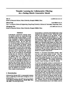
Fig. 1. Illustration of the joint data in text retrieval and collaborative filtering. (a) Querydocument joint data in text retrieval (reproduced from [Robertson et al. 1982]). (b) User-item joint data in collaborative filtering.

between the concepts of users and items in CF and the concepts of documents and queries in information retrieval. Like Robertson et al. [1982] did for documents and queries in information retrieval, [Wang et al. 2006b] identified three types of information embedded in the user-item matrix (see also Section 3.3): 1) ratings of the same item by other users; 2) ratings of different items made by the same user, and, 3) ratings of other (but similar) items made by other (but similar) users. This paper explores deeper the usage of these three types of information in a unified probabilistic framework. 3. BACKGROUND This section introduces briefly the user- and item-based approaches to collaborative filtering [Herlocker et al. 1999; Sarwar et al. 2001]. For A users and B items, the user profiles are represented in a A × B user-item matrix X (Fig. 2(a)). Each element xa,b = r indicates that user a rated item b by r, where r ∈ {1, ..., |R|} and |R| is the number of rating scales. if the item has been rated, and elements xa,b = ∅ indicate that the rating is unknown. The user-item matrix can be decomposed into row vectors, X = [u1 , . . . , uA ]T ua = [xa,1 , . . . , xa,B ]T , a = 1, . . . , A corresponding to the A user profiles ua . Each row vector represents the item ratings of a particular user. As discussed below, this decomposition leads to user-based collaborative filtering. Alternatively, the matrix can be represented by its column vectors, X = [i1 , ..., iB ] ib = [x1,b , ..., xA,b ]T , b = 1, ..., B corresponding to the ratings by all A users for a specific item b. As will be shown, this representation results in item-based recommendation algorithms. ACM Journal Name, Vol. V, No. N, Month 20YY.


(a)

·

7

(b)

(c)

(d)

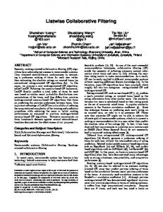
Fig. 2. (a) The user-item matrix (b) User-based approaches (c) Item-based approaches (d) Combining user-based and item-based approaches. 3.1 User-based Collaborative Filtering User-based collaborative filtering predicts a test user’s interest on a test item based on the ratings of this test item from other similar users. Ratings by more similar users contribute more to predicting the test item rating. The set of similar users can be identified by employing a threshold on the similarity measure or just selecting the top-N most similar users. In the top-N case, a set of top-N users similar to test user a, Tu (ua ), can be generated by ranking users in order of their similarities: Tu (ua ) = {uc |rank su (ua , uc ) < N },

(1)

where su (ua , uc ) is the similarity between users a and c. Cosine similarity and Pearson Correlation are popular similarity measures in collaborative filtering, see e.g. [Breese et al. 1998]. The similarity could also be learnt from training data [Cheung and Tian 2004; Jin et al. 2004]. Notice that the formulation in Eq. 1 assumes that xc,b = ∅ =⇒ su (ua , uc ) = 0, i.e., the users that did not rate the test item b are not part of the top-N similar users Tu (ua ). Consequently, the predicted rating x ba,b of test item b by test user a is computed ACM Journal Name, Vol. V, No. N, Month 20YY.

8

·

Jun Wang et al.

as

X x ba,b = xa +

su (ua , uc ) · (xc,b − xc )

uc ∈Tu (ua )

X

su (ua , uc )

,

(2)

uc ∈Tu (ua )

where xa and xc denote the average rating on all the rated items, made by users a and c, respectively. Existing methods differ in their treatment of unknown ratings from similar users (i.e. the value xc,b = ∅). Missing ratings can be replaced by a 0 score, which lowers the prediction, or the average rating of that similar user could be used (mean imputation) [Breese et al. 1998; Herlocker et al. 1999]. Alternatively, [Xue et al. 2005] replaces missing ratings by an interpolation of the user’s average rating and the average rating of his or her cluster (k-NN imputation). Fig. 2(b) illustrates the user-based approach. In the figure, each user profile (row vector) is sorted and re-indexed by its similarity towards the test user’s profile. Notice in Eq. 2 and in Fig. 2(b) user-based collaborative filtering takes only a small proportion of the user-item matrix into consideration for recommendation, i.e. only the known test item ratings by similar users are used. We refer to these ratings as the set of ‘similar user ratings’ (the blocks with upward diagonal pattern in Fig. 2(b)): SURa,b = {xc,b |uc ∈ Tu (ua )}. For readability, we drop the subscript a, b of SURa,b in the remainder of the paper. 3.2 Item-based Collaborative Filtering Item-based approaches such as [Deshpande and Karypis 2004; Linden et al. 2003; Sarwar et al. 2001] apply the same idea using the similarity between items instead of users. The unknown rating of a test item by a test user is predicted by averaging the ratings of other similar items rated by this test user. Ratings from more similar items are weighted stronger. Formally, X si (ib , id ) · xa,d x ba,b =

id ∈Ti (ib )

X

si (ib , id )

,

(3)

id ∈Ti (ib )

where item similarity si (ib , id ) can be approximated by the cosine measure or Pearson correlation [Linden et al. 2003; Sarwar et al. 2001]. To remove the difference in rating scale between users when computing the similarity, [Sarwar et al. 2001] has proposed to adjust the cosine similarity by subtracting the user’s average rating from each co-rated pair beforehand. Like the top-N similar users, a set of top-N similar items towards test item b, denoted as Ti (ib ), can be generated according to: Ti (ib ) = {id |rank si (ib , id ) < N }

(4)

Fig. 2(c) illustrates the item-based approaches. Each item (column vector) is sorted and re-indexed according to its similarity towards the test item in the user-item matrix. Eq. 3 shows that only the known similar item ratings by the test user are taken into account for the prediction. We refer to the ratings used in the item-based ACM Journal Name, Vol. V, No. N, Month 20YY.


·

9

approach as the set of ‘similar item ratings’ (the blocks with downward diagonal pattern in Fig. 2(c)): SIRa,b = {xa,d |id ∈ Ti (ib )}. Again, for simplicity, we drop the subscript a, b of SIRa,b in the remainder of the paper.

3.3 Combining User-based and Item-based Approaches When the ratings from these two sources are quite often not available, predictions are often made by averaging ratings from ‘not-so-similar’ users or items. Therefore, relying on SU R or SIR ratings only is undesirable. In order to improve the accuracy of prediction, [Wang et al. 2006b] proposed to combine both user-based and item-based approaches. Additionally, we pointed out that the user-item matrix contains useful data beyond the previously used SUR and SIR ratings. As illustrated in Fig. 2 (d), the similar item ratings made by similar users may provide an extra source for prediction. They are obtained by sorting and re-indexing rows and columns according to their similarities towards the test user and the test item respectively. In the remainder, this part of the matrix is referred to as ‘similar user item ratings’ (the grid blocks in Fig. 2(d)): SUIRa,b = {xc,d |uc ∈ Tu (ua ), id ∈ Ti (ib ), c 6= a, d 6= b}. The subscript a, b of SUIRa,b is dropped. Their similarity towards the target rating xa,b , denoted as sui (xa,b , xc,d ), can be calculated as follows: 1

sui (xa,b , xc,d ) = p

(1/su (ua , uc ))2 + (1/si (ib , id ))2 (5)

where a Euclidean dis-similarity space is adopted such that the resulting combined similarity is lower than either of them. Now we are ready to combine these three types of ratings in a single collaborative filtering method. We treat each element of the user-item matrix as a separate predictor. Its confidence for the prediction is then estimated based upon its similarity towards the test rating. We then predict the test rating by averaging the individual predictions weighted by their confidence. Formally, X c,d x ba,b = pa,b (xc,d )Wa,b , (6) xc,d

where

pa,b (xc,d ) = xc,d − (xc − xa ) − (xd − xb )

(7)

can be treated as a normalization function when predicting rating xa,b from rating xc,d . xa and xc are the average ratings by user a and c, and xb and xd are the c,d average ratings of item b and d. For each test rating xa,b , Wa,b acts as a unified ACM Journal Name, Vol. V, No. N, Month 20YY.

10

·

Jun Wang et al.

weight matrix to combine the predictors from the three different sources:  su (ua ,uc ) P  xc,d ∈ SUR  su (ua ,uc ) λ(1 − δ)   xc,d ∈SUR      Psi (ibs,id(i) ,i ) (1 − λ)(1 − δ) xc,d ∈ SIR i b d c,d xc,d ∈SIR , Wa,b =  sui (xa,b ,xc,d )  P  δ x ∈ SUIR c,d  sui (xa,b ,xc,d )   xc,d ∈SUIR    0 otherwise

(8)

where λ ∈ [0, 1] and δ ∈ [0, 1] control the importance of the different rating sources. This combination of ratings can be considered as two subsequent steps of linear interpolation. First, predictions from SUR ratings are interpolated with SIR ratings, controlled by λ. Next, the intermediate prediction is interpolated with predictions from the SUIR data, controlled by δ. The second interpolation corresponds to smoothing the SIR and SUR predictions with SUIR ratings as a background model. A bigger λ emphasizes user correlations, while smaller λ emphasizes item correlations. When λ equals one, the algorithm corresponds to a user-based approach, while λ equal to zero results in an item-based approach. Tuning parameter δ controls the impact of smoothing from the background model (i.e. SUIR). When δ approaches zero, the fusion framework becomes the mere combination of user-based and item-based approaches without smoothing from the background model. 4. PROBABILISTIC RELEVANCE PREDICTION MODELS This section re-formulates the collaborative filtering problem in a probabilistic framework. Motivated by the probabilistic relevance models proposed in text retrieval domain [Robertson and SparckJones 1976; Lafferty and Zhai 2003; Ponte and Croft 1998], we introduce the concept of “relevance” into collaborative filtering. By analogy with the relevance models in text retrieval, the collaborative filtering problem can be solved by answering the following basic question: what is the probability that this item is relevant to this user, given his or her profile? To answer this question, firstly, let us define a sample space of relevance: ΦR and let R be a random variable over the relevance space ΦR . Unlike the commonly used binary relevance in text retrieval, in our case here, the relevance is multiple-valued. Thus, let us define that ΦR has multiple values, which are observed from the rating data: ΦR = {1, ..., |R|}, where |R| is the number of rating scales. From now on, each known element (xa,b 6= ∅) in the user-item matrix is treated as an observation of this multiple-scaled relevance. Secondly, let U be a discrete random variable over the sample space of user id ’s: ΦU = {u1 , ..., uA } and let I be a random variable over the sample space of item id ’s: ΦI = {i1 , ..., iB }, where A is the number of users and B the number of items in the collection. In other words, U refers to the user identifiers and I refers to the item identifiers. We then denote P as a probability function on the joint sample space ΦU × ΦI × ΦR . A prediction model thus can be built by estimating the conditional probability of the rating P (R|U, I), given the specified user and item identifiers. The expectation of the unknown rating of a given item I = ib from a given user ACM Journal Name, Vol. V, No. N, Month 20YY.


·

11

U = ua can be formulated as follows: x â,b =

|R| X

rP (R = r|I = ib , U = ua )

(9)

r=1

For simplicity, R = r, U = ua , and I = ib are denoted as r, ua , and ib , respectively. Before proceeding, let us highlight how the current formulation using ratings differs from the probabilistic model that we have proposed before for log-based CF [Wang et al. 2006a]. In the log-based model, relevance variable r is binary, observed as “the file is (not) downloaded” or the “web-site is (not) visited”. In that case, ΦR has binary values ‘relevant’ r and ‘non-relevant’ r. The resulting model is a ranking model, and does not attempt to predict the rating. Conversely, the model proposed in this paper is a rating prediction model, that is especially targeted to rating-based CF; i.e., the model predicts directly the number of stars that a user would assign to the test item. 4.1 Three Different Relevance Models The way to estimate P (r|ib , ua ) plays an important role in our model. Three different models, namely user-based relevance, item-based relevance and unified relevance models can be derived if we apply the Bayes’ rule differently:  P (ua |r,ib )P (r|ib ) User-based Relevance  P (ua |ib )  P (ib |r,ua )P (r|ua ) Item-based Relevance P (r|ib , ua ) = (10) P (ib |ua )   P (ua ,ib |r)P (r) Unified Relevance P (ib ,ua ) Each of the three derivations represents a different view of the problem. We shall see that the former two models (i.e. the user-based relevance model and the item-based relevance model) represent a partial view of the collaborative filtering problem while the third model unifies these partial views. 4.1.1 derive:

User-based Relevance Model. Applying the first factorization in Eq. 9, we |R| X P (ua |r, ib )P (r|ib ) r P (ua |ib ) r=1 P|R| rP (ua |r, ib )P (r|ib ) = r=1 P (ua |ib ) P|R| rP (ua |r, ib )P (r|ib ) , = Pr=1 |R| r=1 P (ua |r, ib )P (r|ib )

x â,b =

(11)

where the final prediction relies on two probabilities: 1) The conditional probability P (ua |r, ib ) builds up a user space model conditioned on the target item and the rating. It measures how probable a user may rate item ib as rating r and thus it is the preference model of a user. 2) The probability P (r|ib ) measures how likely the target item ib may be rated as rating r. It can be regarded as a rating prior or the rating model. Clearly, together the product of the two probabilities serves as a weight for each rating scale r. The denominator, a sum over the different rating ACM Journal Name, Vol. V, No. N, Month 20YY.

12

·

Jun Wang et al.

P|R| scales r=1 P (ua |r, ib )P (r|ib ), serves as a normalization factor. To simplify the notation, we choose ri to denote the joint event between r and i (i.e. rating for item i). Hence P (ua |r, ib ) is written as P (ua |rib ). Notice that, in the user preference model (P (ua |r, ib )) in Eq. 11, users are defined by their ‘user identifiers’ in the user id space. To be able to make a prediction for a new user, we need to build a feature representation and use it to relate the new user to the training users. For this, instead of putting users in the original user id space, we represent them by their ratings. So, P (ua |rib ) = P (ua |rib ), where the vector ua = [xa,1 , . . . , xa,B ]T denotes the B item ratings from user a. Unrated items can be filled with the average rating value, or taken as a constant value 0 instead. Substituting user identifiers by their rating vectors in Eq. 11 gives: P|R|

rP (ua |rib )P (r|ib )

x â,b = Pr=1 |R|

r=1

P (ua |rib )P (r|ib )

(12)

4.1.2 Item-based Relevance Model. We derive the following equation the same way, by factorizing P (r|ua , ib ) in Eq. 9 as P (ib |ua , r)P (r|ua )/P (ib |ua ): P|R| rP (ib |r, ua )P (r|ua ) x â,b = Pr=1 |R| r=1 P (ib |r, ua )P (r|ua )

(13)

To simplify notation, let ru denote the joint event between r and u (i.e., the rating from user u), and P (ib |r, ua ) be written as P (ib |rua ). Following the same line of reasoning as for the user case above, an item can be represented using each user’s rating as a feature, such that P (ib |rua ) = P (ib |rua ) where the vector ib = [x1,b , . . . , xA,b ]T denotes the A user ratings for item b. Again, the missing ratings can be replaced by the average rating value or by a constant value 0. This gives P|R| x â,b = Pr=1 |R|

rP (ib |rua )P (r|ua )

r=1

P (ib |rua )P (r|ua )

(14)

Probability P (ib |rua ) conditions the item space on the user’s rating. It expresses how probable an item is rated as value r by user ua , and can be regarded as the preference model of an item. The probability P (r|ua ) measures how likely the target user ua may provide a rating as value r. It can be treated as a rating prior, or, the target user’s rating model. Obviously, the final weight for each rating scale is a product between these two models. The summation over different rating scales P|R| r=1 P (ib |rua )P (r|ua ) in the denominator serves as a normalization factor. 4.1.3 Unified Relevance Model. Let us now introduce the unified relevance model. We derive from Eq. 9: P|R| x â,b = Pr=1 |R|

rP (ua , ib |r)P (r)

r=1

P (ua , ib |r)P (r)

ACM Journal Name, Vol. V, No. N, Month 20YY.

(15)


·

13

Table I.

Probabilities in the three different models. Preference Model Rating Model User-based Relevance P (ua |rib ) P (r|ib ) Item-based Relevance P (ib |rua ) P (r|ua ) Unified Relevance P (ua , ib |r) P (r)

Analogous to the two other derivations, we use ratings as features to represent users and items, respectively: P (ua , ib |r) = P (ua , ib |r). P|R| rP (ua , ib |r)P (r) x â,b = Pr=1 (16) |R| r=1 P (ua , ib |r)P (r) The preference model now involves the user and item together. Table I summarises the three different models derived from Eq. 9 (Eq. 12, 14 and 16). The weights to average the rating scales equal the product of a preference model and a rating model. Since the three models are derived from the same root, they are probabilistically equivalent, but the different factorizations lead to the different probability estimations, so statistically they are inequivalent. 4.2 Probability Estimation The next problem is how to estimate the probabilities listed in Table I. Because the rating space is one-dimensional, the densities for the rating models can be estimated by simply counting the frequency of the co-occurrences. For the density estimations of the preference models however, the high dimensionality of the user feature space and the item feature space complicates matters. Here, we use the nonparametric Parzen-window method for density estimation (also known as kernel density estimation). This approach extrapolates the density from the sample data. The main advantage over a parametric approach is that we do not have to specify the model structure a priori, but may determine it from the data itself. 4.2.1 Density Estimation for Rating Models. Estimating the three rating models corresponds to counting the co-occurrence frequencies of the three joint events: P c(ua , ib , r) |Srua | P (r|ua ) = P ib = (17a) |Sua | ib ,r c(ua , ib , r) P |Srib | c(ua , ib , r) P (r|ib ) = P ua = |Sib | ua ,r c(ua , ib , r) P P (r) = P

ua ,ib

c(ua , ib , r)

ua ,ib ,r c(ua , ib , r)

=

|Sr | , |S|

(17b)

(17c)

where c(ua , ib , r) ∈ {0, 1} denotes the co-occurrence function; c(ua , ib , r) equals one if user ua rated item ib as r, zero otherwise. S(·) denotes the set of observed samples where event (·) happened, |S(·) | its cardinality. For example, Srib denotes the set of observed samples with event (R = P r, I = ib ), so |Srib | corresponds to the number of times that this event happened, ua c(u Pa , ib , r). S denotes the entire set of observed samples and |S| its size, equal to ua ,ib ,r c(ua , ib , r). ACM Journal Name, Vol. V, No. N, Month 20YY.

14

·

Jun Wang et al.

Table II. Commonly used Parzen kernel functions. 1 Rectangular 2 for |x| < 1, 0 otherwise Triangular 1 − |x|for|x| < 1, 0 otherwise 15 2 2 Biweight 16 (1 − x ) for |x| < 1, 0 otherwise 2 √1 e−x /2 Gaussian 2π √ √ Bartlett - Epanechnikov 34 (1 − x2 /5)/ 5 for |x| < 5, 0 otherwise 4.2.2 Density Estimation for Preference Models. Given some observed samples of a population, the Parzen-window method extrapolates the data to the entire population by averaging from neighborhood observed samples. The neighborhood samples are selected and weighted according to some pre-defined Parzen kernel window functions. Usually, the Parzen kernel function is required to be non-negative and symmetric, and it should integrate to one. Table II lists the most commonly used Parzen kernels for univariate data. The multi-dimensional feature spaces in which users and items are represented require a multivariate Parzen kernel (denoted as K(y)), that can be obtained using a product of univariate Parzen kernels: K(y) =

Q Y

Kq (yq ),

(18)

q=1

where y = [y1 , ..., yQ ] is a Q-dimensional vector. Kq is the univariate Parzen kernel function for the qth dimension. We assume all univariate kernels to be equal: Kq = K. The product of the univariate Parzen kernel assumes that the dimensions (features) are locally independent (where the locality is defined by the univariate Parzen kernel function K). Pluging in the bandwidth parameter, we have: Q 1 yq y 1 y1 yQ 1 Y K( ), K( ) = K( , ..., ) = Q Q Q h h h h h h q=1 h

(19)

where to reduce the complexity of the model, we have assumed the bandwidth of each Parzen window to be equal in each dimension, defined as h. First, take preference models P (u|rib ) and P (i|rua ) in the user-based and the item-based relevance derivations. Both depend on a single feature vector; either the user vector u or the item vector i. Directly applying the Parzen-window method by using the univariate product Parzen kernel, we obtain the following equations for the density estimations ([Duda et al. 2001]): P (u|rib ) =

P (i|rua ) =

1 |Srib | 1 |Srua |

X

1

u0 ∈Sri

hu

B

K(

u − u0 ) hu

(20a)

b

X i0 ∈Srua

1 i − i0 K( ), A hi hi

(20b)

where hi and hu are the bandwidth window parameters for the user vector and item vector, respectively. ACM Journal Name, Vol. V, No. N, Month 20YY.


·

15

Next, consider the preference model in the unified relevance case, P (ua , ib |r). Probability estimation requires a density in the joint user-item feature space. We employ a product of two univariate kernel density estimators: X 1 u − u0 1 i − i0 1 P (ua , ib |r) = K( ) K( ), (21) |Sr | 0 0 hu hi hu B hi A (u ,i )∈Sr

where Sr denotes the set of observed samples when event (R = r) happens, while P |Sr | denotes its size, equal to ua ,ib c(ua , ib , r). The kernel density estimation can be interpreted as a mixture of the component densities with an equal weight. Each mean of the component densities is located in the place where the neighborhood observation is available. The shape of the density is controlled by the Parzen kernel window function and its bandwidth parameter. Thus, the final prediction can be expressed by the summation over the Parzen kernels which are situated in the location of the neighborhood samples. 4.3 Rating Predictions Consider now the problem of rating prediction in the user-based relevance model. Substituting the user-based rating model of Eq. 17a and the user preference model of Eq. 20a in the generic user-based relevance model of Eq. 12 gives: ³P ´ |Sr | P|R| ib 1 1 u−u0 r ) K( 0 B r=1 |Sri | u ∈Sri hu hu |Sib | b b x â,b = P (22) ´ |Sr | ³P |R| ib 1 u−u0 1 K( ) 0 B r=1 |Sr | u ∈Sr hu |Si | hu ib

ib

b

Cancelling out the factors |Srib | and |Sib | simplifies Eq. 22 to: ´ P|R| ³ P u−u0 u0 ∈Sri K( hu ) r=1 r b ³P ´ x â,b = P |R| u−u0 K( ) 0 u ∈Sr r=1 hu

(23)

ib

Combining the outer summation over r with the inner over u0 completes our approach to perform rating prediction using the user-based relevance model: P u−u0 0 u0 ∈Sib ru ,ib K( hu ) (24) x â,b = P , u−u0 u0 ∈Si K( hu ) b

where u0 ∈ Sib denotes the (other) users who have rated item ib , and, ru0 ,ib denotes the rating of user u0 for item ib . Rating prediction in the item-based relevance model is derived analogously: P i−i0 0 i0 ∈Sua ri ,ua K( hi ) (25) x â,b = P , i−i0 i0 ∈Sua K( hi ) where i0 ∈ Sua denotes the other items rated by user ua , and, ri0 ,ua denotes the rating of user i0 for item ua . Finally, rating prediction with the unified relevance model: P i−i0 u−u0 0 0 (u0 ,i0 )∈S ru ,i K( hu )K( hi ) (26) x â,b = P , u−u0 i−i0 (u0 ,i0 )∈S K( hu )K( hi ) ACM Journal Name, Vol. V, No. N, Month 20YY.

16

·

Jun Wang et al.

where ru0 ,i0 denotes the rating of user u0 for item i0 . Again, S denotes the entire sample set S = S1 ∪ · · · ∪ S|R| . The next step specifies the Parzen-window kernel function K and its bandwidth parameter h. A common choice is to use the Gaussian density function as the univariate Parzen kernel function: Y − ||yq ||2 ||y||2 1 1 1 y − 2h2 e 2h2 K( ) = e = √ √ (27) Q Q hQ h ( 2πh) ( 2πh) q Substituting the Gaussian Parzen-window in the above equations results in the following preference models: P (ua |rib ) =

1 √ |Srib |( 2πhu )B

1 √ P (i|rua ) = |Srua |( 2πhi )A P (ua , ib |r) =

1 |Sr |

X

X

e

−

||u−u0 ||2 2hu 2

u0 ∈Sri

b

X

e

−

||i−i0 ||2 2hi 2

i0 ∈Srua ||i−i0 ||2 ||u−u0 ||2 1 − − √ e 2hu 2 e 2hi 2 ( 2πhu )B ( 2πhi )A

√

(u0 ,i0 )∈Sr

(28)

Using these three probability estimates gives the final three equations for rating prediction, corresponding to the three rating prediction models proposed in this paper: User-based Relevance Model: ||u−u0 ||2 P − 2h 2 u u0 ∈Sib ru0 ,ib · e x â,b = 0 2 ||u−u || P − 2h 2 u u0 ∈Si e

(29a)

b

Item-based Relevance Model: ||i−i0 ||2 P − 2h 2 i i0 ∈Sua ri0 ,ua · e x â,b = 0 2 ||i−i || P − 2h 2 i i0 ∈Sua e Unified Relevance Model: P x â,b =

(u0 ,i0 )∈S

ru0 ,i0 · e

P (u0 ,i0 )∈S

e

−

−

(29b)

||u−u0 ||2 2hu 2

||u−u0 ||2 2hu 2

e

−

e

−

||i−i0 ||2 2hi 2

||i−i0 ||2 2hi 2

(29c)

4.4 Cross-validated EM algorithm Previous studies have shown that the type of Parzen kernel function has usually only a marginal effect on the quality of density estimation; however, the choice of the bandwidth window parameter h has a significant influence [Skurichina 1990]. In our case, the two bandwidth window parameters hu and hi need to be tuned to ACM Journal Name, Vol. V, No. N, Month 20YY.


·

17

the data. If their value is too small, the estimated density is a collection of sharp peaks positioned at the sample points, such that the density estimation still suffers from the data sparsity. If their value is however too large, the density estimate is over-smoothed, such that the underlying structure in the data is not preserved in the estimated density. The optimal bandwidth parameters can be found by maximising the following cross-validated (leave the estimated u or i out) likelihood function [Duin 1976]: Y X i − i0 1 1 u − u0 1 ˆ u, h ˆ i = arg max h K( ) A K( ) B |Sr − 1| 0 0 hu hu hi hi hu ,hi 0 0 (u,i)∈Sr

(u ,i )∈Sr ∧(u 6=u)∧(i 6=i)

(30) This maximisation problem can be solved using the iterative Expectation maximisation (EM) algorithm [Dempster et al. 1977; Paclik et al. 2000]. For readability, we give the final expectation (E) and maximisation (M ) steps here but leave the detailed derivation for Appendix A: —E step: e

P (t) (u0 , i0 |u, i) =

−

||u−u0 ||2 2hu 2

P u0 6=u,i0 6=i

—M step:

s h(t+1) u

=

1 X B|Sr | u,i

(t+1) hi

s =

X

e

−

−

e

||i−i0 ||2 2hi 2

||u−u0 ||2 2hu 2

e

−

||i−i0 ||2 2hi 2

(31a)

P (t) (u0 , i0 |u, i)(||u − u0 ||2 )

(31b)

P (t) (u0 , i0 |u, i)(||i − i0 ||2 )

(31c)

u0 6=u,i0 6=i

1 X A|Sr |

X

u,i u0 6=u,i0 6=i

where t equals the number of the iteration. 4.5 A Generalised Distance Measure The univariate Gaussian Parzen kernel used in the previous measures the distance between users and item using Euclidean or L2 distance (||u − u0 ||2 and ||i − i0 ||2 ). However, many alternative distances could be considered. A previous study [Herlocker 2000] shows that the mean-squared difference is less effective for collaborative filtering than Pearson correlation and the cosine measure. We could of course adapt our framework using a different Parzen-window function, and try to set things up such that the density estimation is based on the cosine measure instead of Euclidean distance. Ideally, we would however like to generalise the Parzen-window density estimation from the specific distance measure of our choice. We can achieve this goal using the mathematics that has become known as the kernel trick in the machine learning community [Schölkopf and Smola 2001]. Notice that the term kernel will refer to a different kernel function than the one in the Parzen-window density estimation; to avoid confusion, we use the term projection kernel. The kernel trick transforms any algorithm that solely depends on the dot product between two vectors, by replacing this dot product with the application of ACM Journal Name, Vol. V, No. N, Month 20YY.

18

·

Jun Wang et al.

the projection kernel. It has been proven (based on the Moore-Aronszajn-Theorem) that a positive definite projection kernel determines a unique function φ such that: K(y, y0 ) =< φ(y), φ(y0 ) >,

(32)

where denotes the dot product. This equation is often used without knowing the exact form of function φ; it suffices to know that it exists and is defined uniquely. Schölkopf has shown that an even larger class of projection kernels (referred to as conditionally positive definite functions) satisfies Eq. 32 [Schölkopf 2000]. Now, basic linear algebra allows us to relate the Euclidean distance in projected space to the application of a projection kernel in user- or item-space: ||φ(y) − φ(y0 )||2 X = (φ(yi ) − φ(yi0 ))2 i

X = {φ(yi )2 − 2φ(yi )φ(yi0 ) + φ(yi0 )2 } i

X

=

i

2

φ(yi ) +

X

φ(yi0 )2

−2

i

X

(33)

φ(yi )φ(yi0 )

i

= < φ(y), φ(y) > + < φ(y0 ), φ(y0 ) > −2 < φ(y), φ(y0 ) > =K(y, y) + K(y0 , y0 ) − 2K(y, y0 ) Using a length-normalised projection kernel for which K(y, y) = 1 gives ||φ(y) − φ(y0 )|| = K(y, y) + K(y0 , y0 ) − 2K(y, y0 ) = 2 − 2K(y, y0 )

(34)

So, computing a Euclidean distance in projected space is equivalent to using a positive definite projection kernel K to compute distances in the original space. This property allows us to perform Parzen-window density estimation with the Gaussian kernel in the projected space, without actually knowing the function φ (which is however defined uniquely by the choice of the projection kernel). In the remainder, we use the length-normalised dot product as the projection kernel (also known as the cosine kernel, denoted as Cos(y, y0 ) [Liu et al. 2004]): K(y, y0 ) = Cos(y, y0 ) = √

< y, y0 > < y, y >< y0 , y0 >

(35)

Thus, we have: ||φ(y) − φ(y0 )||2 = 2 − 2Cos(y, y0 )

(36)

In this specific case, function φ is actually known and corresponds to vector normalization: y y = pP φ(y) = √ (37) 2 < y, y > i (yi ) Eq. 36 demonstrates that the cosine dissimilarity measure is indeed equivalent to a Euclidean distance measure in the projected space. So, we can perform Parzenwindow density estimation with a Gaussian window function in the projected space: Kh (φ(y), φ(y0 )) =

0 )||2 0) J 1−Cos(y,y J − ||φ(y)−φ(y 2h2 h2 e = e− , h h

ACM Journal Name, Vol. V, No. N, Month 20YY.

(38)


·

19

Table III. Relationship between the choice of Parzen kernel, bandwidth parameters and the projection kernel and CF algorithms. Bandwidth Parameters

Parzen Kernel

hu ∈ IR

Gaussian

hi = ∞

Bartlett-Epanechnikov

hi ∈ IR

Gaussian

hu = ∞


hu ∈ IR

Gaussian

hi ∈ IR


Projection Kernel Cosine Null Cosine Null Cosine Null Cosine Null Cosine Null Cosine Null

CF Algorithm User-based Relevance Model (Eq. 40a) Eq. 29a and PD ([Pennock et al. 2000]) User-based method, VS ([Breese et al. 1998]) User-based, Ringo ([Shardanand and Maes 1995]) Item-based Relevance Model (Eq. 40b) Eq. 29b Item-based method, VS ([Sarwar et al. 2001]), Item-based Relevance Model, Euclidean Distance Unified Relevance Model (Eq. 40c) Eq. 29c ([Wang et al. 2006b]) and ([Hu and Lu 2006]) Unified Relevance Model, Euclidean Distance

where J is a normalization factor to obtain a Parzen window function, i.e., to satisfy Z 0) J − 1−Cos(y,y h2 e dy = 1 (39) y h 1−Cos(y,y0 )

h2 It is easy to show that J ∈ IR since h1 e− is bounded in the y space. By employing Eq. 38 instead of Eq. 27, we integrate the cosine similarity measure into our final rating prediction models:

User-based Relevance Model: 1−Cos(u,u0 ) P − h2 u u0 ∈Sib ru0 ,ib e x â,b = 1−Cos(u,u0 ) P − h2 u e u0 ∈Si

(40a)

b

Item-based Relevance Model: P x â,b =

i0 ∈Sua

ri0 ,ua e

P i0 ∈Sua

e

−

1−Cos(i,i0 ) h2 i

−

(40b)

1−Cos(i,i0 ) h2 i

Unified Relevance Model: P x â,b =

(u0 ,i0 )∈S

r

−

u0 ,i0

P (u0 ,i0 )∈S

e

e

1−Cos(u,u0 ) h2 u

1−Cos(u,u0 ) − h2 u

e

e

−

−

1−Cos(i,i0 ) h2 i

1−Cos(i,i0 ) h2 i

(40c)

Estimation of parameters hu and hi follows the same procedure as in the Euclidean distance case, see Appendix A. 4.6 Discussion The General Framework The proposed combination of Parzen-window kernel density estimation with the relevance models provides a general framework for colACM Journal Name, Vol. V, No. N, Month 20YY.

20

·

Jun Wang et al.

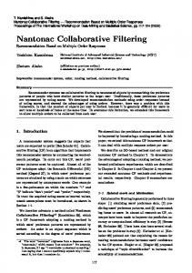
laborative filtering. The three rating prediction models listed in Eq. 40a, 40b and 40c, show how the final predictions are expressed by summations over rating influences from the neighborhood samples (from user neighbors Eq. 40a, item neighbors Eq. 40b, or both the user and item neighbors Eq. 40c). Three factors determine the influence of the neighborhood samples on the prediction: the type of Parzen kernel, its bandwidth parameters, and, the distance of the neighborhood samples from the sample to be predicted. The Parzen kernel smoothes the prediction, while the projection kernel allows us to select the right distance measure. Different choices for the bandwidth parameters, the Parzen-window kernel function or the projection kernel lead to different approaches to collaborative filtering. For instance, it is easy to see that using the Bartlett-Epanechnikov kernel (given in Table II) with hi equal to one and hu to ∞ simplifies the unified relevance prediction formula in Eq. 26 to the item-based cosine similarity method (using Eq. 36): P ri0 ,ua Cos(i, i0 ) i0 ∈S x â,b = P ua (41) 0 i0 ∈Sua Cos(i, i ) Table III summarises how the general framework can be specialised to various previously known approaches. The User-based and Item-Based Views The user-based relevance model and item-based relevance model represent two different views for the problem. In the user-based relevance model, we fix the target item ib . Conditioned on it, we build up a user representation P (ua |ib , r) (See Fig. 3 (a)). This is analogous to the document-oriented approaches in text retrieval [Maron and Kuhns 1960; Lafferty and Zhai 2003], where queries represented by the terms are conditioned on the fixed target document model P (Q|db , r).1 Conversely, in the item-based relevance model, we fix the target user ua and conditioned on it, we build up an item representation P (ib |ua , r) (see Fig. 3 (b)). This is analogous to the query-oriented approach in text retrieval [Robertson and SparckJones 1976], where documents D are represented by the terms and these representations are conditioned on the fixed query terms P (D|qa , r).2 The Unified View Unlike the above two models, the unified relevance model in Eq. 40c however provides a rather completed and unified view of the problem. In this model, we do not fix the two variables: user and item. Instead, we construct a unified model that relies on both the user representation and the item representation P (ua , ib |r) (see Fig. 3 (c)). The model is solved by applying the kernel density estimation and it provides a practical solution for the unification advocated in [Robertson et al. 1982]. It can also be treated as a generalised version of the similarity fusion approach to CF [Wang et al. 2006b]. The model intuitively provides a unified probabilistic framework to fuse userbased and item-based approaches. In addition, the ratings from similar users for similar items (the SUIR ratings) are employed to smooth the predictions. We highlight the relationship to the similarity fusion method of [Wang et al. 2006b] by 1 In

the language modelling literature, the document-oriented approach is also referred to as a query-generation model. 2 The query-oriented approach is also known as a document-generation model for information retrieval. ACM Journal Name, Vol. V, No. N, Month 20YY.


·

21

dividing the entire set of observations S into three sets: the ratings from test user Su , the ratings for test item Si , and the remaining ratings Su¯,¯ı . Eq. 40c gives 1−Cos(i,i0 ) ´ 1−Cos(u,u0 ) − 1³ X − h2 h2 u i x â,b = ru0 ,i0 e e H (u0 ,i0 )∈S (42) ´ X X 1³ X = ru0 ,i E + ru,i0 F + ru0 ,i0 G , H 0 0 0 0 (u ,i)∈Si

(u,i )∈Su

(u ,i )∈Su ¯ ,¯ ı

where H is a normalization factor equal to 1−Cos(i,i0 ) 1−Cos(u,u0 ) X − − h2 h2 u i e e

(43)

(u0 ,i0 )∈S

The three types of ratings ru0 ,i , ru,i0 and ru0 ,i0 that contribute to the prediction are precisely the similar user ratings (SUR), the similar item ratings (SIR) and the similar user towards similar item ratings (SUIR). E, F and G determine three weights for averaging these ratings: E=e F =e G=e

−

1−Cos(u,u0 ) h2 u

−

1−Cos(i,i0 ) h2 i

−

1−Cos(u,u0 ) h2 u

(44) e

−

1−Cos(i,i0 ) h2 i

The bandwidth parameters hu and hi control the width of the kernel function. A small bandwidth value leads to spiky estimates while larger bandwidth values over-smooth the observations with data from far away samples. The bandwidth parameters also balance the contributions from the user side and the item side. A small hu emphasizes user correlations, and a small hi emphasizes the item correlations (see also the experiments corresponding to Fig. 9 and Fig. 10). When hu approaches ∞, the unified relevance model corresponds to item-based collaborative filtering, while an hi of ∞ results in user-based recommendation. 4.7 Computational Complexity This section discusses the scalability of our collaborative filtering framework. The computational complexity of the framework consists of the amount of time needed for building the model (i.e. the EM estimation of the two bandwidth parameters and the probability estimations), and that of making online recommendations for a new user from the model. The EM algorithm is only needed during the model building phase. Thus there are no iterative steps required in the online recommendation phase. Furthermore, we propose an efficient method to calculate the kernel-based similarities, largely reducing the computational complexity. 4.7.1 Offline Computation. In the model building phase, Eq. 29c simplifies the probability estimations to the calculations of the kernel-based similarities. That is, for any user pair and item pair, we need to calculate their kernel similarities −

||u−u0 ||2

−

||i−i0 ||2

e 2hu 2 and e 2hi 2 , respectively. To make the calculation efficient, we decompose them into the distance measure part (||u − u0 || or ||i − i0 ||) and the kernel ACM Journal Name, Vol. V, No. N, Month 20YY.

22

·

Jun Wang et al. −

•

−

•

smoothing part (e 2hu 2 or e 2hi 2 ). Thus, model building consists of two steps: first computing two distance (dis-similarity) matrices and then estimating the two bandwidth parameters. For each element in the matrix, we require either B arithmetic operations for the user-to-user distance or A arithmetic operations for the item-to-item distance. In total the upper bound of the computational complexity is O(A2 B + B 2 A), which is roughly equal to a sum of the complexity of a user-based method [Herlocker et al. 1999] and that of an item-based method [Sarwar et al. 2001]. Since the data is extremely sparse, with a proper data structure, the computation can be largely reduced. This paper proposes to use two inverted files, respectively indexing users and items about their ratings. When we calculate the distances, for instance, for a given user, we do not need to go through all other users about their agreement on all items. Instead, we first from the user indexing file get the set of items that he or she has rated, and then go through these items, accessing a set of users who have rated any of these items (from the item index file). By doing this, not only do we exclude the users who do not share any commonly-rated item from the computations, we also restrict the operations to those items that the two users both rated. Thus the overall computation is much faster than the original user-based or item-based methods, only requiring a linear time complexity that approximately equals O((A + B)mn), where m is the average number of user ratings per item and n is the average number of item ratings per user. In addition, it is unnecessary to store all the non-zero elements in the distance matrices, as we shall see in our experiment (Fig. 8) that keeping only the top-N nearest user neighbors and the top-N nearest item neighbors improves prediction accuracy, where N is typically in the range of (30...70). Once we have the user (item) distance matrix that stores the top-N nearest neighbors, the EM estimation of hi and hu becomes a relatively simple task because it essentially averages the user or item distance from the distance matrices in an iterative manner (see Eq. 31). For the sake of time efficiency, the E step and M step can be computed together, where the computational complexity in each iteration is given by O(ABN 2 ) because we need to average all possible user-item pair (A × B operations) and for each pair, we need to access N × N neighbors. In practice, the complexity of the EM algorithm can be further reduced by sub-sampling both training users and training items; our additional experiments (not reported) verified that a small amount of training user-item pairs is sufficient to get the stable and accurate estimations of hu and hi . We shall see in our experiment (Fig. 4) that the EM algorithm converges fast, and a small number of iterations (3-5) suffices to get relatively stable estimations in the tested data sets. 4.7.2 Online Computation. The online recommendation can be computed very efficiently if we again utilize both the user and item indexing files. For a new user, the computational complexity of his or her kernel similarity towards other users is approximately given as O(mn) because on average we access his or her m rated items and for each of these items access n users who rate it. The final prediction corresponds to a weighted average from the ratings of the top-N nearest items and the top-N nearest users, resulting in a computational complexity of O(N 2 ), which is independent of the number of users and items. ACM Journal Name, Vol. V, No. N, Month 20YY.


(a)

(b)

·

23

(c)

Fig. 3. Illustration of the three different models. (a) User-based Relevance Model. (b) Item-based Relevance Model. (c) Unified Relevance Model.

Table IV.

Characteristics of the test data sets.

Num. of Users Num. of Items Avg. Num. of Rated Item Per User Avg. Num. of User Rating Per Item Sparsity Rating Scales

MovieLens 1 943 1682 106.0 59.5 6.30% 5(1-5)

MovieLens 2 500 1000 87.7 43.9 8.77% 5(1-5)

EachMovies 1 2,000 1,648 90.0 114.2 5.7% 6(1-6)

EachMovies 2 10,000 1,648 96.3 611.0 6.11% 6(1-6))

5. EXPERIMENTS 5.1 Data Sets We experimented with two movie rating data sets: the MovieLens [DataSet a] and the EachMovie [DataSet b] data sets. The MovieLens data set was collected by the GroupLens group through the MovieLens web site during the period from September 1997 through April 1998. It contains ratings by 943 users for 1682 movies (items). Each user has rated at least 20 movies. The rating scale takes values from 1 ( the lowest rating) to 5 (the highest rating). In addition, to compare with other approaches we also adopt a widely-used subset [Si and Jin 2003], which contains 500 users and 1000 movies (items), where each user has rated at least 40 items. The EachMovie data set was collected by the Digital Equipment Research Center during the period from 1995 to 1997. The rating scale was originally indicated as the values from 0 (no star), 0.2 (one star) and up to 1 (five stars). For consistency with the MovieLens data set, we transformed the rating scales to the values 1 − −6, with 1 being the lowest rating (i.e., no star) and 6 being the highest one (i.e., five stars). To compare with other approaches, we adopt the two subsets described in [Si and Jin 2003] and [Xue et al. 2005], which respectively contain 2,000 users and 10,000 users. In both cases, each user has rated as least 40 items. The basic characteristics of these two data sets with the different size are summarised in Table IV. We mainly use the MovieLens 1 data set to conduct empirical analyses on our models while using the other sets to conduct the performance tests. ACM Journal Name, Vol. V, No. N, Month 20YY.

24

·

Jun Wang et al.

5.2 Evaluation Protocols For testing, we assigned the users in the data set at random to a training user and a test user set. Users in the training set are used as the basis for making predictions, while our test users are considered the ground truth for measuring prediction accuracy. Each test user’s ratings have been split into a set of observed items and one of held-out items. The ratings of the observed items are input for predicting the ratings of the held-out items (the test items). To improve our measurements, each of the experimental setups has been repeated 20 times with different random seeds. For consistency with experiments reported in the literature, e.g., [Jin et al. 2004; Sarwar et al. 2001; Xue et al. 2005]), we report our results using the mean absolute error (MAE) evaluation metric. MAE corresponds to the average absolute deviation of predictions to the ground truth data, for all test item ratings and test users: P |xa,b − x ba,b | M AE =

a,b

, (45) L where L denotes the number of tested ratings. A smaller value indicates a better performance. 5.3 Results 5.3.1 Parameter Estimation. This section conducts the experiments on the EM estimation for the parameters hu and hi . We first test the convergence behavior of the cross-validated EM method using MovieLens set 1. To reduce redundancy, we only show the estimation results when we randomly select 400 users as the training data. Notice that the estimation over other number of training users behaves consistently. Fig. 4 shows that the EM algorithm converges in few iterations (about 3) to the optimal bandwidth parameters (h2u = 0.79 (Fig. 4(a)) and h2i = 0.49 (Fig. 4(b))) with respect to the log likelihood object function (Fig. 4 (c)). Repeating this experiment with different random initial values of hu and hi (have a relatively large standard deviation in the figures), the EM algorithm converges to (almost) the same optimal values (have a relatively small standard deviation in the figures). Observe that the obtained bandwidth parameter hu is relatively larger than the parameter hi . To explain this result, we investigate the influence of the distribution of neighboring vectors on the parameter estimation. In our models, both the user distance and item distance are measured by the cosine distance, i.e. 1 − Cos(u, u0 ) and 1 − Cos(u, u0 ) (Eq. 40a–40c). Fig. 5 plots the distributions of the top-50 nearest users and items as a histogram of 10 bins in the distance range of [0, 1]. It shows that, on average, the user distances are larger than the item distances. So, estimating the user density needs a bigger bandwidth parameter to smooth from the neighborhood than that of the item density. To show the sensitivity of the two bandwidth parameters regarding to the recommendation performance, we plot the value of the bandwidth parameter (either hu or hi ) against the MAE measurement in Fig. 6. It shows that the two bandwidth parameters are relatively stable in a wide range regarding to the MAE performance. Also, comparing the optimal bandwidth parameters with the ones shown in Fig. 4 we can see that, although the EM algorithm uses a different objective function ACM Journal Name, Vol. V, No. N, Month 20YY.

·

Unified Relevance Models for Rating Prediction in Collaborative Filtering 0.9

0.9

0.8

0.8

0.7

0.7

0.6

0.6

0.5

0.5

0.4

0.4

0.3

0.3

0.2

25

0.2 h2u

0.1

0

0.5

1

1.5

2

2.5 Iterations

(a)

3

3.5

4

4.5

h2i 0.1

5

0

0.5

1

1.5

2

h2u

2.5 Iterations

(b)

3

3.5

4

4.5

5

h2i

−2

−3

−4

−5

−6

−7

−8

Log Likelihood −9 0.5

1

1.5

2

2.5

3 Iterations

3.5

4

4.5

5

5.5

(c) Log Likelihood Objective Function

0.9

0.9

0.8

0.8

0.7

0.7

0.6

0.6

Probability

Probability

Fig. 4. Convergence behavior of the cross-validated EM algorithm: Using the cosine projection kernel (400 training users in the MovieLens 1 data set).

0.5

0.4

0.5

0.4

0.3

0.3

0.2

0.2

0.1

0.1

0

0

0.1

0.2

0.3

0.4

0.5 0.6 Cosine Distance

(a)Top-50 User

0.7

0.8

0.9

1

0

0

0.1

0.2

0.3

0.4

0.5 0.6 Cosine Distance

0.7

0.8

0.9

1

(b)Top-50 Item

Fig. 5. Distribution of cosine distance in the MovieLens data set (400 training users in the MovieLens 1 data set). ACM Journal Name, Vol. V, No. N, Month 20YY.

·

Jun Wang et al.

1.02

1.02

1

1

0.98

0.98

MAE

MAE

26

0.96

0.94

0.96

0.94

0.92

0.92 h2u

0.9

0

0.1

0.2

0.3

0.4

0.5 h2u

0.6

0.7

0.8

0.9

h2i 0.9

1

0

0.1

0.2

0.3

0.4

0.5 h2i

0.6

0.7

0.8

0.9

1

(b)h2i

(a)h2u

Fig. 6. The sensitivity of the two parameters regarding to the MAE measurement (the remaining 543 test users in the MovieLens 1 data set). 5000

h2 i

0.95

Average True Top−N ×(N+2)

0.9

4000

4000

0.85

2

2

hu

2000

hi

3000 0.7


0.75

0.6 2000


0.8

0.8

1000

0.4 h2u Average True Top−N ×(N+2) 0

50

100

150 TopN

200

250

0 300

(a) h2u vs. top-N

0

50

100

150 TopN

200

250

0 300

(b) h2i vs. top-N

Fig. 7. The impact of the neighbor size on the parameter estimation. (400 training users in the MovieLens 1 data set).

(log likelihood), it does give a reasonably good estimation of the two bandwidth parameters in terms of the MAE. In practice, recommendation systems make a trade-off between prediction accuracy and run-time system efficiency by pre-selecting the top-N nearest user neighbors (SUR) and the top-N nearest item neighbors (SIR). These form a rating pool, extended with the top-N ×N nearest similar user to similar item neighbors (SUIR). In total, we would have N × (N + 2) neighbors. However, only the neighbors whose ratings are available in the pool contribute to the predictions. Clearly, the parameter N affects the parameter estimation and therefore also the performance of our fusion methods. Fig. 7 plots the estimated parameter values of hu and hi under different neighbor sizes, where the x axis represents the size of the pre-selected top-N and the left y axis corresponds to the estimated value of the parameter (hu in Fig. 7(a) and hi in Fig. 7(b)). The right y axis shows the ‘true’ number of SUR, SIR and SUIR within the pool that have to be retrieved to obtain non-empty ratings for estimation. The graph shows that for low values of N , both parameters hu ACM Journal Name, Vol. V, No. N, Month 20YY.


·

27

0.86

0.84

MAE

0.82

0.8

0.78

0.76

0.74

50

100

150 TopN

200

250

300

Fig. 8. The MAE performance under different neighbor size (the remaining 543 test users in the MovieLens 1 data set). 1

0.66 Test Item Sparsity: < 15 Test Item Sparsity: < 20 Test Item Sparsity: < 25 Test Item Sparsity: < 30 Test Item Sparsity: < 40 Test Item Sparsity: < 60 Test Item Sparsity: < 100 Test Item Sparsity: < No constraint

0.95

Test Item Sparsity: < 15 Test Item Sparsity: < 20 Test Item Sparsity: < 25 Test Item Sparsity: < 30 Test Item Sparsity: < 40 Test Item Sparsity: < 60 Test Item Sparsity: < 100 Test Item Sparsity: < No constraint

0.64

0.62

0.6

0.9 0.58

0.85

0.56

0.54 0.8 0.52

0.5 0.75 0.48

0.7

5

10 15 Num. of Given Rating Per Test User

(a) h2u Fig. 9.

20

0.46

5

10 15 Num. of Given Rating Per Test User

20

(b) h2i

The optimal bandwidth parameters with different user sparsity.

and hi increase fast. This shows that the new ratings introduced by increasing the top-N contribute to improve the prediction accuracy, such that the corresponding Parzen-window should cover the newly introduced ratings (so, the bandwidth parameters increase). Gradually however, this increase diminishes, because a large top-N introduces more and more noisy ratings. Consequently, the parameter values converge and the Parzen-window excludes the distant ratings from the estimation process. Fig. 8 displays the MAE of the unified relevance model under different neighbor sizes, to illustrate the effect of the estimated parameters on prediction accuracy. The optimal result corresponds to N ' 50. The error increases only slowly with larger values of N , due to the fact that the Parzen-window reduces the effect of the noisy (distant) neighbors when they are introduced. We select 50 as the optimal choice of N for the subsequent experiments. 5.3.2 Sparsity. This section investigates the effect of data sparsity on the performance of our collaborative filtering methods in more detail. For this, we set up ACM Journal Name, Vol. V, No. N, Month 20YY.

·

28

Jun Wang et al.

1

0.66 Test User Sparsity: 5 Test User Sparsity: 10 Test User Sparsity: 15 Test User Sparsity: 20

0.95

Test User Sparsity: 5 Test User Sparsity: 10 Test User Sparsity: 15 Test User Sparsity: 20

0.64

0.62

0.6 0.9 0.58

0.85

0.56

0.54 0.8 0.52

0.5 0.75 0.48

0.7

20

30

40 50 60 70 Max Num. of Given Rating Per Test Item

(a) Fig. 10.

80

90

0.46

100

1.1

1.1

1.05

1

1

0.95

0.95

0.9

0.9

0.85

0.85

0.8

0.8

0.75

0.75

10

15 20 25 Num. of Given Rating Per Test User

30

35

40

0.7

0

1.1

1.1

1.05

1

1

0.95

0.95

0.9

0.9

0.85

0.85

0.8

0.8

0.75

0.75

50 60 70 Max Num. of Given Rating Per Test Item

80

90

5

10


30

35

40

UnifiedRM UserRM ItemRM

1.15

1.05

40

100

(b) Num. of user rating per Item: < 100


1.15

30

90


(a) Num. of user rating per Item: < 20

0.7 20

80

h2i

1.15

1.05

5

40 50 60 70 Max Num. of Given Rating Per Test Item

The optimal bandwidth parameters under different item sparsity. UnifiedRM UserRM ItemRM

0

30

(b)

1.15

0.7

20

h2u

100

(c) Num. of item rating per user: 2

0.7 20

30

40


80

90

100

(d) Num. of item rating per user: 38

Fig. 11. Performance of the three derived models under different sparsity in the MovieLens 1 data set.

the following configurations: 1) Test User Sparsity: vary the number of items rated by test users in the observed set, e.g. 5, 10, or 20 ratings per user. 2) Test Item ACM Journal Name, Vol. V, No. N, Month 20YY.

·

Unified Relevance Models for Rating Prediction in Collaborative Filtering 1.4

1.4 UnifiedRM UserRM ItemRM

1.35

1.3

1.3

1.25

1.2

1.2

1.15

1.15

1.1

1.1

1.05

1.05

1

1

0.95

0.95

0

5

10


30

35


1.35

1.25

0.9

29

40

0.9

0

(a) Num. of user rating per item: < 20

10


30

35

40

(b) Num. of user rating per item: < 100

1.4

1.4 UnifiedRM UserRM ItemRM

1.35

1.3

1.3

1.25

1.2

1.2

1.15

1.15

1.1

1.1

1.05

1.05

1

1

0.95

0.95

30

40


80

90

(c) Num. of item rating per User: 2


1.35

1.25

0.9 20

5

100

0.9 20

30

40


80

90

100

(d) Num. of item rating per User: 38

Fig. 12. Performance of the three derived models under different sparsity in the EachMovie 1 data set.

Sparsity: vary the number of users who have rated test items in the held-out set, e.g. less than 15, 20, 25 (denoted as ‘< 15’, ‘< 20’, or ‘< 25’), or, unconstrained (denoted as ‘No constraint’). Notice that the configurations of the user sparsity and the item sparsity are not completely symmetrical in order to reflect the practical situation. The first experiment investigates the effect of data sparsity on parameter estimation using the EM algorithm. We use the different sparsity configurations: user sparsity: number of given ratings per user (5, 10, 15, 20) and item sparsity: maximum number of user rating per item (