criteria for the uniqueness of limit cycles when they exist for a specialized class of ... corrected a flaw in the proof of Cheng's [5] main theorem and extended the.
Uniqueness of Limit Cycles in Cause-Type Models of Predator-Prey Systems YANG KUANG* AND H. I. FREEDMAN+ Department of Mathematics, University of Alberta, Edmonton, Canada T6G ZGI Received 27 March 1987; revised I7 September I987
ABSTRACT This
paper
deals
with
the question
of uniqueness
of limit
cycles
in predator-prey
systems of Gause type. By utilizing several transformations, these systems are reduced to a generalized Lienard system as discussed by Cherkas and Zhilevich and by Zhang. As a consequence, criteria Cheng and is related
for the uniqueness of limit cycles are derived, which include results of to results in Liou and Cheng. Several examples are given to illustrate
our results.
1.
INTRODUCTION
Since the papers of May [19] and Albrecht, Gatzke, and Wax [l], an outstanding problem in mathematical modeling of ecological systems has been that of determining conditions which guarantee uniqueness of limit cycles in predator-prey models. In two dimensions it is well known that there can be no limit cycles in models of competitive or cooperative systems. Further, it is known for predator-prey systems that the existence and stability of a limit cycle is related to the existence and stability of a positive equilibrium. We assume such a positive equilibrium exists, for otherwise the predator population tends to extinction [8, Chapter 41. If the equilibrium is asymptotically stable, there may exist limit cycles, the innermost of which must be unstable from the inside, and the outermost of which must be stable from the outside. If limit cycles do not exist in this case, the equilibrium is globally asymptotically stable. Conditions for this last situation to occur are given by Cheng, Hsu, and Lin [6], Goh [13], Hsu [17], and Freedman and So
191. There are various techniques for establishing the existence of limit cycles, (see, e.g. [8, 10, 111). However, we emphasize that criteria for their uniqueness are virtually unknown. *Research partially supported by a Killam Postgraduate Scholarship at the University of Alberta. ‘Research partially supported by the Natural Sciences and Engineering Research Council of Canada, Grant No. NSERC A4823. MATHEMATICAL
BIOSCIENCES
88:67-84
Wlsevier Science Publishing Co., Inc., 1988 52 Vanderbilt Ave., New York, NY 10017
67
(1988)
0025-5564/88,‘$03.50
YANG KUANG AND H. I. FREEDMAN
68
If the positive equilibrium exists and is unstable, there must occur at least one limit cycle. In 1972 May [19] claimed that under the Kolmogoroff conditions, a “unique,” stable limit cycle must exist. In response to this Albrecht et al. [l] constructed a predator-prey system satisfying the Kolmogoroff conditions (except for the self-contradiction contained therein) for which there are uncountably many periodic solutions filling an annular region between two limit cycles. In 1981 Cheng [5] published a result giving criteria for the uniqueness of limit cycles when they exist for a specialized class of predator-prey models. Subsequently, Liou and Cheng [18] have corrected a flaw in the proof of Cheng’s [5] main theorem and extended the class of predator-prey models for which the results are valid. In this paper, by a different technique, we are able to obtain criteria for uniqueness of limit cycles in the case of an unstable positive equilibrium for a more general class of Gause-type predator-prey models, which include those studied by Liou and Cheng [18] as a special case, and which allow for the possibility of mutual interference among predators. The technique we use is to transform our model to a generalized Lienard system as studied by Zhang [25] and to note that aside from the usual predator-prey assumptions, one additional assumption is required for the uniqueness of limit cycles. Although the class of predator-prey models considered in this paper is not the most general Kolmogorov type, it certainly includes many models utilized by experimental and field biologists in studying predator-prey interactions. Models of this type were introduced by Gause, Smaragdova, and Witt [12] in 1936 to help analyze paramecium-didinium interactions. Since then, various forms of these models (both continuous and discrete) have been utilized by Armstrong [2-41, Hassell [15], Hassell and May [16], and Rosenzweig [20-221. In the next section we describe the class of models that we consider. In Section 3, we describe the generalize Lienard system and results on it. Section 4 describes our transformation and main theorems. This is followed by a section giving examples to illustrate our results. The final section contains a discussion. We complete the proof of a required theorem of Cherkas and Zhilevich [7] in the appendix. 2.
THEMODEL We consider
a class of Gause predator-prey
models of the form
x(0)
2
0,
Y(O)2 0,
(2.1)
where ‘= d/dt, and where g, E, 7, p, q are sufficiently smooth so that existence, uniqueness, and continuability for all positive t are satisfied for
UNIQUENESS
69
OF LIMIT CYCLES
initial-value problems. We think of x(t) and y(t) as representing the prey and predator populations, respectively, at given time t > 0. The following assumptions are consistent with models of predator-prey systems for x, y > 0. (Hl):
g(0) > 0; there exists K > 0 such that g(x) > 0 on 0 d x < K, g(K) = 0, g(x) < 0 on x > K.
(H2): (H3): (H4): (H5):
E(O) = 0, p (0) = 0, n(O) = 0, q(0) = 0,
NY) p’(x) n’(y) q’(x)
’ 0. > 0. > 0. > 0.
Note that in the special case that t(y) = n(y) = y, q(x) = cp(x), this is precisely the intermediate class of predator-prey models discussed in [8, Chapter 41. We remark that a new feature of such predator-prey models is incorporated into the case when g’(0) > 0. This represents a prey population which can exhibit an accelerated population specific growth rate for small values of population as a strategy to avoid extinction. Clearly the system (2.1) has equilibria at E,,(O,O) and E1( K,O). In order for there to exist a positive equilibrium of the form E*(x*, y*) the equation q(x) = y must have a positive solution [which by (H5) will be unique]. Further, this value x* must be smaller than K, for otherwise y* is not defined. Hence we assume (H6):
There exists 0 < x* < K such that q(x*) = y.
In order that y* be defined we further assume (H7):
lim, _ m KY) ’ x*g(x*)/P(x*).
Then y* = [-‘(x*g(x*)/p(x*)). librium.
H ence,
E* is a unique
positive
equi-
Clearly E, is a saddle point, stable in the y-direction and unstable in the x-direction. Assuming (H6), El is also a saddle point, stable along the x-axis. In order to discuss the stability of E*, we compute the variational matrix about E*, denoted by J*, and get
H(x*)
J*= dY*)q'(x*)
-
s“(Y*)P(x*) 0
I
(2.2)
’
where H( x*) = x*g’( x*) + g( x*) - x*g6;;)$‘x*’
.
(2.3)
70
YANG KUANG AND H. I. FREEDMAN
Similarly to [8, Chapter 41, the eigenvalues of J* have real positive (negative) parts if H(x*) is positive (negative), implying the instability (asymptotic stability) of E*. Throughout the remainder of this paper, we assume that E* exists and is unstable (so that there is at least one positive limit cycle surrounding E*). By the criterion of Rosenzweig and MacArthur [8, Chapter 41, this is equivalent to assuming x=x*‘o. 3.
RESULTS
ON A GENERALIZED
LIENARD
SYSTEM
The following theorem was proved by L. A. Cherkas and L. I. Zhilevich in 1969 [7]. Since complete detail of proof was not given in the original paper, and since we require a different format than that of [7], we have included its proof in the appendix of this paper. THEOREM Let
3.1 (L. A. CHERKAS
the generalized
AND L. I. ZHILEVICH)
Lienard system dx TZ=
-[‘P(Y)+F(x)l, (3.1)
$=h(x) satisfy
the following
conditions:
(1) xh( x) > 0 when x + 0, and ycp( y) > 0 when y + 0. (2) cp( y) is monotonically f(x)
increasing,
F(0) = 0, and f (0) < 0 ( > 0), where
= F’(x). (3) There exist real numbers a and p such that the function fi(x)
(3.2)
=f(x)+h(x)[a+PF(x)l
has simple zeros x1 -C 0 and x2 > 0, and f,( x) < 0 ( > 0) in x1 < x < x2. (4) Outside x1 < x < x1 the function f,(x)/h(x) does not decrease (does not increase). (5) AN the limit cycles contain the interval x1 < x < x2 on the x-axis. Then the system
(3.1) has at most one limit cycle, which, if it exists, is stable
(unstable).
From the proof of this theorem (see Appendix) (4) can be modified to
we observe that condition
(4’) All the limit cycles are contained in the interval x3 Q x Q x4, where x3 C x1 < 0 < x2 < xq
UNIQUENESS
OF LIMIT CYCLES
and the function fi (x)/h 0, dl/dt > 0, dk-‘/dt Now, we rewrite (4.6) as follows:
> 0 and dl-‘/dt
> 0.
-[~(f-‘tu)+Y*)-5tY*)l b=-y+q(k-‘(u)+x*). By comparing
(4.7)
(4.7) with (3.1), we have the following correspondences:
h(x)
++-y+q(k-‘(u)+x*),
T(Y)
+~-‘(~)+v*)-aY*)9
Hence, if we define h(u)=-y+q(k-‘(u)+x*), v(u)
=6(l-‘(u)+r*)-5(r*),
F(u)
=cE(y*)-[k-‘(u)+x*]
(4.8) ;‘c;::;;;;;:;,
we may observe that the following hold: (1) h(O)=-y+q(x*)=O; h’(u)>O,hence Similarly, ucp(u) > 0 when u + 0.
uh(u)>Owhenu#O.
UNIQUENESS OF LIMIT CYCLES (2)
We have
cp,(v)
=
dww+Y*) d(l_‘(u)+y*)
i.e., I& 0) is monotonically increasing. (3) cp(v)+F(u)=Oisdefinedforall (4) We have
dF(O)
dF(u)
-=
du
UE(-MJ,+IX).
. d(k-‘(4+x*) du
d(k-‘(u)+x*)
from (HS) and the fact (5) For such models, must lie inside the strip must he inside the strip (6) We have
f(u)
dl-‘(v) > dv ’ 0
.~
0. it is known [8, Ch. 41 that the limit cycles of (2.1) 0 < x < K, 0 < y < co. Hence the limit cycles of (4.7) - co < u < k(K), - co -Cu -C + co.
=F’(u)
=
dF( u) d[k-‘(u)+x*]
dk-‘( du
u) .
(4.9)
Since the system (2.1) has a unique limit cycle if and only if the system (4.7) has a unique limit cycle, we have the following general theorems. Corresponding to Theorem 3.1, we obtain THEOREM
4.1
In the system (4.7), let there exist real numbers a and j3 such that
fl(u) =fb)+h(u)b+BF(u)l has simple zeros u1 < 0 < u2, and fi( u) < 0 in u1 d u d u2, and let the function fi (u)/h (u) be nondecreasing in ( - co, u,), ( u2, k(K)). Moreover, suppose all the limit cycles contain the interval u1 Q u < u2 on the u-axis. Then system (2.1) has exactly one limit cycle which is globally asymptotically stable with respect to the set {(x, y) ] x > 0, y > 0} \ {E*}. Corresponding THEOREM
to Theorem 3.2, we obtain
4.2
Suppose in the system (4.7) f (u)/h ( u ) is nondecreasing in ( - 00 ,O) and (0, k(K)). Then the system (2.1) has exactly one limit cycle which is globally asymptotically stable with respect to the set {(x, y ) 1 x > 0, y > 0} \ { E * } .
14
YANG KUANG AND H. I. FREEDMAN
In most systems discussed in the ecological literature, I;(y) = q(y) = y. In this case, we have the following simplifications:
u=k(X),
U=l(Y)=hy
(4.10)
Y= y*e” - y*.
(4.11)
or
Hence (4.7) can be rewritten as
y*-[k-‘(u)+x*]
g(k-‘(24)+x*)
p( k-‘( u) + x*)
-(y*e” -‘*)’ (4.12)
I+-y+@‘(u)+x*). Note that 1(=
/0xP(s+x*) a5
=k(X),
X-k-‘(u)
Hence du -= dX
1 P(X+x*)
’
or
dk;;u)=$=p(X+x*)
=P(k-‘(u)+x*),
(4.13)
and f(u)
=
=-
_@’u,
d(k
‘(u)+x*)
.P( k-‘( u) + x*)
xf(x)+g(x)-xg(x)po
p’(x)
.
(4.14)
x=k-‘(u)+x*
Therefore f( u)/h (u) is nondecreasing if and only if
Since
d(k&
+ x*>
f(k-l(u)+x*) A( k-‘( u) + x*)
*p(k-l(u)
+ x*)’
UNIQUENESS f( u)/h(
75
OF LIMIT CYCLES
u) is nondecreasing if and only if
d
-xi
> I
xg’(x)+d+*g(x)~
I
0.
-Y+q(x)
(4.15)
Hence, we have the following version of Theorem 4.2 for the system i =
x&T(x)- yp(x>,
2
0,
(4.16)
y(0) > 0.
L=Y[-Y+dx)l, THEOREM
x(0)
4.2
Suppose in the system (4.16)
d X
xg’(x)+dx)-xdx)# -y+t(x)
I
GO
(4.17)
in 0 Q x < x* and x* < x 4 K. Then the system (4.16) has exactly one limit cycle which is globally asymptotically stable with respect to the set {(x, y ) 1x > 0, y>O}\{E*}. Note.
In the case q(x) = cp(x), (4.17) is equivalent to
i.e.,
[cp(x)-YlP(X)(
$g)“-YPt(x)(
yf$)‘O,
y(O)=y,>O,
discussed in [23], where r, k, m, a, a, Do are positive constants. ing results are known (see [23]): (1) Solutions
of (5.1) are positive and eventually
uniformly
The follow-
bounded.
(2) Denote
if
m>D,
(a) If m Q Do, or if m > Do and KG A, then the equilibrium E,(K,O) is asymptotically stable and lim, --to. s(t) = K, lim, _ m y(t) = 0. (b) If A < K Q a +2X, the equilibrium E*(X, y*) is asymptotically stable, and lim,,, s(t) = A, limr_m r(l) =y*, where y* = (ra/m) (1 - X/K)( a + A). (c) If K > a + 2A, then (A, y*) is unstable and there exists at least one periodic orbit in the first quadrant of the s - y plane. By using a symmetry argument, Cheng [5] proved that if K > a + 2X, then system (5.1) possesses a unique limit cycle which is stable. The proof is very tedious. However, by employing Theorem 4.3, this result can be obtained
UNIQUENESS
77
OF LIMIT CYCLES
easily. This will be equivalent to proving the following:
(r(l-+)+s(-+)):&-Sk:r(l-+)
(2s+a-K+2s)(s-A)-s(2s+a-K)
1 6o
(5.2)
20
2s2+4Xs-X(a-K)>O
i.e., K > a +2X. The equality holds if and only if K = a +2X. This completes the proof of uniqueness in case (c). Example 2.
We consider the more general model
M”]-4~)m dY X’Y
(5.3)
Cl+_X [ -Y +B(=)m],
where r, y, a, 8, a, m, t9 > 0. In the following calculation, we set 8 = 2,
YANG KUANG AND H. I. FREEDMAN
78 m
=l.
Hence
Suppose (x, JJ) is the unique equilibrium
ax
$=we assume
a-f
-
-=A>0 orx=a/3-y
a+?
Hence
o/3 > y and
X < K, which implies
By the Rosenzweig-MacArthur need
to be increasing
2
x
(
)I
criterion,
a+x
-
(YX
j = (/3/y) rh [l-
- to ensure (x, y) is unstable
=;(a+,)
[
l-
(
$
we
2
)I
xII 2+$+A) i-g120,
at (X, j), i.e., ;
l-
x
[
(
or
3X2 +2ah Without
ap>y.
@
(X/K)‘].
rxl-, [
of (5.3). Then
loss of generality,
- K2 < 0.
(5.4)
we assume K = 1. Then (5.4) becomes 3A2 +2aX O.
(5.6)
Note that D(0) = X > 9, and that D’(x)
=18x2+2(2a-9A)cl!-4ah =2(x-X)(9x+2a).
Hence D’(x) 2 0 for x > X and D’(x) Q 0 for 0 d x d A. Therefore
D(x) >
79
UNIQUENESS OF LIMIT CYCLES
D(A) for x > 0 and D(X) = X(1-2aX -3h*) > 0. This implies under the above assumption that the system (5.3) has a unique limit cycle. We note that the system (5.3) can be transformed into the system considered by Liou and Cheng [18] after a suitable change of variables. Example 3. The following example cannot be transformed into any systems for which uniqueness of limit cycles has been established in previous papers. This is because the prey isocline in this example is not strictly concave down, which is required by Liou and Cheng [18], an essential assumption for their technical analysis to be carried out. We consider dx zt=
,(++2x-X*+X3-$X4),
(5.7)
dy x=yv(-1+x).
and its derivative H(x) =2-2x +3x2 Let 8(x)=:+2x-x2+x3-$x4 - x3 =2+(x-1)-(~-1)~. The interior equilibrium is E(1,2). Further, H’(1) = 2. Hence E(1,2) is unstable and
xH(x)
=x(2-2x+3x2-x3)
x-l
-y+q(x)
and d dx -i
Now
xH(x) -y+q(x)
=-&[x(x-1)*(-3x+4)-2]
let
L(x)=x(x-1)*(-3x+4). We note that when O 0, which contradicts the fact that h, < 0. Now suppose L, is a semistable cycle. Suppose /? > 0 (the argument is similar when /I < 0). We construct a system of equations depending on the parameter y: dx x = - P(Y) - F(x) (A.3) $=h(x), where F(x) F(x)
= i
F(x)+jXy(l-x,)/z([) x2
dl
when
XGX,,
when
x>xr.
(A4
FIG. 2. The systems (A.3) and (3.1). Solid line represents orbits in (3.1), dashed line represents orbits in (A.3).
UNIQUENESS
OF LIMIT
83
CYCLES
Note that the system (A.3) and the system (3.1) are identical in the half and the new system (A.3) forms a family of rotated vector plane xQx,, fields with respect to y in the half plane x > x2, and hence forms a family of generalized rotated vector fields in the whole plane. The function F(x) satisfies all conditions of the theorem. A comparison of the direction fields for (3.1) and (A.3) shows that since L, is supposed to be semistable, the system (3.1) has an orbit arc of the form PIP, P3 (see Figure 2) for sufficiently small y. System (A.3) has an orbit arc PIPiP{. Hence in the region bounded by the curves PI PiP{P, and _L,, the system (A.3) has a limit cycle & with h2 2 0, and inside L, a cycle L, with h, Q 0, i.e., & surrounds z,. But h, < h,. This is a contradiction. Hence L, is stable proving the theorem.
REFERENCES 1
F. Albrecht,
2
Science 181:1073-1074 (1973). R. A. Armstrong, The effects of predator
3
predator-prey stability: A graphical approach, Ecology 57:609-612 (1976). R. A. Armstrong, Fugitive species: Experiments with fungi and some theoretical
4 5
H. Gatzke,
and N. Wax, Stable limit cycles in prey-predator functional
response
considerations, Ecology 57~953-963 (1976). R. A. Armstrong, Prey species replacement along a gradient graphical approach, EcoZogv 60:76-84 (1979).
populations,
and prey productivity
of nutrient
on
enrichment:
A
7
K.-S. Cheng, Uniqueness of a limit cycle for a predator-prey system, SIAM J. Math. Anal. 12:541-548 (1981). K.-S. Cheng, S.-B. Hsu, and S.-S. Lin, Some results on global stability of a predator-prey system, J. Math. Biol. 12:115-126 (1981). L. A. Cherkas and L. I. Zhilevich, Some tests for the absence or uniqueness of limit
8
cycles, Differential Equations 6~891-897 (1970). H. I. Freedman, Deterministic Mathematical Models in Population
6
Dekker, 9 10 11
12 13 14 15 16
New York,
H. I. Freedman
Ecology,
Marcel
1980.
and J. W.-H.
So, Global
stability
chains, Math. Biosci. 76~69-86 (1985). H. I. Freedman and P. Waltman, Perturbation
and persistence
of two dimensional
of simple
food
predator-prey
equations, SIAM J. Appl. Math. 28:1-10 (1975). H. I. Freedman and P. Waltman, Perturbation of two dimensional predator-prey equations with an unperturbed critical point, SIAM J. Appl. Math. 29:719-733 (1975). G. F. Gause, N. P. Smaragdova and A. A. Witt, Further studies of interaction between predator and prey, J. Animal Ecol. 5:1-18 (1936). B.-S. Goh, Global stability in a class of predator-prey models, Bull. Math. Biol. 40:525-533 (1978). P. Hartman, Ordinary Differential Equations, Wiley, New York, 1964. M. P. Hassell, The Dynamics of Arthropod Predator-Prey Systems, Princeton, U.P., Princeton, 1978. M. P. Hassell and R. M. May, Stability in insect host-parasite models, J. Animal Ecol. 42:693-726 (1973).
84
YANG KUANG AND H. I. FREEDMAN
S.-B. Hsu, On the global stability of a predator-prey system, Math Eiosci. 39:1-10 (1978). 18 L.-P. Liou and K.-S. Cheng, On the uniqueness of a limit cycle for a predator-prey system, to appear. 19 R. M. May, Limit cycles in predator-prey communities, Science 177900-902 (1972). 20 M. L. Rosenzweig, Why the prey curve has a bump, Amer. Nat. 103:81-87 (1969). 21 M. L. Rosenxweig, Paradox of enrichment: Destabilization of exploitation ecosystems in ecological time, Science 171:385-387 (1971). 22 M. L. Rosenxweig, Evolution of the predator isocline, Evolution 27:84-94 (1973). 23 P. Waltman, Competition Models in Population Biology, SIAM, Philadelphia, 1983. 24 Y.-Q. Ye, S.-L. Cai, L. S. Chen, K.-C. Huang, D.-J. Luo, Z.-E. Ma, E.-N. Wang, M.-S. Wang, X.-A. Yang, and Chi Y. Lo (translator), Theov of Limit Cycles, Amer. Math. Sot., Providence, 1986. 25 Z.-F. Zhang, Proof of the uniqueness theorem of limit cycles of generalized Lienard equations, Appl. Anal. 23163-76 (1986). 17