MODARES JOURNAL OF ELECTRICAL ENGINEERING,VOL.12,NO.3, FALL 2012
Stable Limit Cycles Generating in a Class of Uncertain Nonlinear Systems: Application in Inertia Pendulum Ali Reza Hakimi1, Tahereh Binazadeh2* Received: 2015/9/15
Accepted: 2015/11/22
Abstract This paper considers the problem of stable limit cycles generating in a class of uncertain nonlinear systems which leads to stable oscillations in the system’s output. This is a wanted behavior in many practical engineering problems. For this purpose, first the equation of the desirable limit cycle is achieved according to shape, amplitude and frequency of the required output oscillations. Then, the nonlinear control law is designed such that the phase portrait of the closed-loop system includes this stable limit cycle. The design of controller is based on the Lyapunov stability theorem which is suitable for stability analysis of the positive limit sets (the stable limit cycle is a positive limit set for the nonlinear dynamicl system). The proposed robust controller consists of two parts: nominal control law and additional term which guarantees the robust performance and vanishing the effect of uncertain terms. Finally, to show the applicability of the proposed method, an inertia pendulum system (with parametric uncertainties in its dynamical equations) is considered and the robust output oscillations are achieved by creating the desirable limit cycle in the close-loop system. Keywords: Positive limit set, Stable oscillations, Robust limit cycle, Lyapunov redesign method. Introduction Generation of stable limit cycles is one of the most famous areas in the control engineering. Stable limit cycles create an oscillatory behavior in the time response of state variable in the nonlinear systems. Stable oscillations are desired behavior in many practical engineering problems like: buck-boost converters, switching power supplies [1,2], walk cyclic pattern [3,4], boom-bust cycles [5,6] and catalytic hyper cycles [7]. Two main approaches have been proposed in literature to create a stable limit cycle in the phase trajectories of the nonlinear systems. In the first approach, limit cycle stabilization is converted to
1. M.Sc. student Department of Electrical and Electronic Engineering, Shiraz University of Technology, Shiraz, Iran
[email protected]
output tracking problem by tracking of the periodic reference signals. For this purpose, the error signal (i.e., the output deviation from the time-varying reference signal) and its derivatives up to the relative degree of system are defined as error vector. Then, by constructing the error dynamical system, the tracking problem is converted to asymptotic stabilization of the time-varying error dynamical system. In this method, the periodic reference signal should be smooth enough and its derivations up to the relative degree of system should be generated. In this way, several robust nonlinear and fuzzy controllers are proposed for different dynamical systems such as underactuated and feedback linearizable systems [8,9]. Another approach is based on the stability analysis of posititve limit sets and extends the Lyapunov stability theorems from the stability analysis of the equilibrium points to stability analysis of the limit sets [10]. In this aproach, selecting the appropriate Lyapunov function is related to the shape of limit cycle and there is no need to generate the time varying reference signal and its derivatives. Based on this approach, the control law may be designed to create a stable limit cycle (as a positive limit set) in the closed-loop system. Authors of [11-13], designed such control laws for special classes of nonlinear systems using different techniques of nonlinear control such as CLF, passivity, backstepping and so on. In these references, the nominal systems are considered and the designed controllers are not robust against uncertainties and external disturbances. However, it is important to note that in modeling of the physical systems, there are uncertain terms due to uncertainty in the parameters, external disturbances or simplification of the model. This paper deals with generating robust stable output oscillation by robust orbital stabilization of a class of uncertain nonlinear systems in the presence of uncertainties and external disturbances. For this purpose, first, by designing an appropriate nonlinear control law, the stable limit cycle is created in the nominal nonlinear system. Then, an additional state feedback term is designed by considering the uncertain terms, such that the overall state feedback controller guarantees generating of a stable limit cycle in the actual closed-loop uncertain nonlinear system. At the end, to examine the applicability of the proposed method, the robust stable oscillations are created in a pendulum with considering parametric uncertainties. Computer simulations verify the theoretical results. Problem Statemant Consider the following uncertain nonlinear system:
2 . Assistant professor Department of Electrical and Electronic Engineering, Shiraz University of Technology, Shiraz, Iran
[email protected]
1
MODARES JOURNAL OF ELECTRICAL ENGINEERING,VOL.12,NO.3, FALL 2012
x&1 = x 2
x& 2 = f ( x ) + g ( x ) (u + δ ( x , u ) )
(1)
where x ∈ D ⊂ ¡ 2 ,{0} ∈ D is the state vector, u ∈ ¡ is the control input, f : ¡2 → ¡ with f (0) = 0 is a smooth function and g : ¡ 2 → ¡ is a nonzero function in the domain of interest. Also δ (x ,u ) is an unknown function which lumped to gather the model uncertainties and external disturbances. The objective is to design a robust state feedback control u = π (x ) such the trajectories of the closed-loop system attract the prescribed limit cycle S , defined by: S = {x ∈ D ⊂ ¡ 2 : ϕ ( x ) = r 2 }
(2)
where ϕ (x ) is a smooth and continuously differentiable function. The shape of ϕ (x ) and the value of r is effective in the shape, amplitude and frequency of the stable oscillations that create in the output of the closed-loop system. Therefore, ϕ (x ) and r are chosen according to objective to create a desired periodic response in the output of the system. For example, in [14], it declared that if the desirable time response of x 1 (t ) and x 2 (t ) are as follows: x 1d (t ) = A sin ω0t , x 2d (t ) = A ω0 cos ω0t ,
(3)
Then a stable limit cycle with equation ϕ (x ) = r 2 (where r = A ω0 and ϕ (x ) = ω02x 12 + x 22 ), should exist in the phase trajectories of the nonlinear second order system. In the other hand, since limit cycles are a specific kind of positive limit sets, therefore, the stability of limit cycles can be investigated by theorems that conclude stability of limit sets. The following theorem extends the Lyapunov stability theory to stability analysis of limit sets: Theorem 1 [15]: Consider the following nonlinear system: x& = F (x )
(4)
where x ∈ D ⊂ ¡ n . Let S ⊂ D be a closed limit set of (4). If there exists a continuously differentiable function V ( x ) such that: I. It is zero on defined limit set S , II. It is positive in some neighborhood D of S , excluding S itself, III. Its time derivative ( V& (x ) = (∂V / ∂x )F (x ) ) is negative in D ∉ S , Then, the limit set S is a stable limit set.
2
Generating Stable Limit Cycles in the Uncertain Nonlinear Systems This section, considers creating a stable limit cycle in the uncertain nonlinear system (1). For this purpose, first the nominal controller u = k (x ) is designed for the nominal system (i.e., δ (x ,u ) = 0 ), such that the defined limit cycle S is attractive in the closed-loop nominal system. Then, to vanish the effect of uncertainties, the additional term υ ( x ) , is designed based on the Lyapunov redesign method, such that the overall state feedback u = k (x ) + υ ( x ) generates the stable limit cycle S in the closed-loop system (1). Consider the nominal version of nonlinear system (1) as follows: x&1 = x 2 x& 2 = f ( x ) + g (x ) u
(5)
y = cx
The control law u = k (x ) , which generates a stable limit cycle in the phase trajectories of the nominal closedloop system, is given in the following theorem: Theorem 2 [13]: Consider the system (5). the following control input generates the stable limit cycle S in the closed-loop system: u = k (x ) 1 = −f ( x ) − k d ( ϕ ( x ) − r 2 ) ζ ( x ) − η ( x ) g (x )
(
)
(6)
where k d > 0 . Also η (x ) and ζ (x ) are continuous functions that satisfy: ζ (x ) =
∂ϕ (x ) ∂x 2
η (x ) = x 2
∂ϕ (x ) ζ (x ) ∂x 1
(7)
Proof: By putting the controller (6) into (5), the resulted close-loop system is: x&1 = x 2
x& 2 = −k d (ϕ (x ) − r 2 ) ζ (x ) − η (x )
(8)
Consider the Lyapunov function candidate as: V (x ) =
2 1 (ϕ (x ) − r 2 ) 2
(9)
This function satisfies the conditions І and ІІ of Theorem 1. Calculating the V& (x ) along the trajectories of the nominal closed-loop system, one has:
HAKIMI AND BINAZADEH: STABLE LIMIT CYCLES GENERATING IN A CLASS OF UNCERTAIN NONLINEAR SYSTEMS:… ωυ + ωδ ≤ ωυ ( x ) + ω ( ρ ( x ) + k 0 sup υ ( x ) )
∂ϕ ∂ϕ V& ( x ) = (ϕ − r 2 ) x&1 + (ϕ − r 2 ) x& 2 ∂x 1 ∂x 2 =
Consider υ ( x ) as:
∂ϕ (ϕ − r 2 ) x 2 + ∂x 1 ∂ϕ (ϕ − r 2 ) ( − k d (ϕ − r 2 )ζ − η ) ∂x 2
(10)
= ηζ (ϕ − r 2 ) − ηζ (ϕ − r 2 ) − k d ζ 2 (ϕ − r 2 ) 2 = − k d ζ (ϕ − r ) 2
2 2
υ (x ) = − β ( x )
ω = − β (x )sgn(ω ) ω
Consequently:
x&1 = x 2
V& = − k d ζ 2 (ϕ − r 2 ) 2 + ωυ + ω δ
(11)
Consider the same Lyapunov function that proposed for the nominal system in (9) as a Lyapunov function candidate for the uncertain system. Differentiating this function along the trajectories of the closed loop system (11) then: ∂V ( x ) ∂V ( x ) V& = x&1 + x& 2 ∂x 1 ∂x 2 =
∂V ∂V x2 + ( −k d (ϕ − r 2 )ζ − η + g (υ + δ ) ) (12) ∂x 1 ∂x 2
= − k d ζ 2 (ϕ − r 2 ) 2 +
∂V g (υ + δ ) ∂x 2
(16)
where β (x ) is a smooth function and it is chosen such that,
Evidently, V (x ) is descending when ζ (x ) ≠ 0 and ϕ (x ) − r 2 ≠ 0 simultaneously. Also, it is invariant when ζ (x ) = 0 or ϕ (x ) − r 2 = 0 . In [13], it is deduced that assuming the closed-loop system is detectable with respect to the output ζ (x ) and unstable at the origin and using LaSalle's invariant theorem, the condition ІІІ in Theorem 1 is also satisfied for all solutions that not initialized at the origin. ■ Now consider the uncertain system (1) (i.e., δ ≠ 0 ). In this case, an additional term will be added to the previous control law to create robust manner. Substituting the control input u = k ( x ) + υ ( x ) in this system results in: x& 2 = f ( x ) + g ( x ) ( k ( x ) + υ ( x ) + δ ( x , u ) )
(15)
β (x ) ≥
ρ (x ) 1− k 0
(17)
Thus sup υ ( x ) = β (x ) and: ωυ + ωδ ≤ ωυ (x ) + ρ (x ) ω + k 0 sup υ (x ) ω ≤ − β (x ) ω + ρ (x ) ω + k 0 β (x ) ω = − β (x )(1 − k 0 ) ω + ρ (x ) ω
(18)
≤ − ρ (x ) ω + ρ (x ) ω =0
(19)
≤ − k d ζ 2 (ϕ − r 2 ) 2
Thus, with the control law (16), the derivative of V ( x ) along trajectories of the closed-loop system (11) is negative and all conditions of Theorem 1 are satisfied. Therefore S is a stable limit cycle for system (11) and the following robust state feedback control law guarantees robust attraction of the trajectories of the closed loop system (11) to limit cycle S in the presence of uncertainties and external disturbances. u = k (x ) + υ ( x ) 1 = −f (x ) − k d (ϕ (x ) − r 2 ) ζ (x ) − η (x ) (20) g (x ) − β (x )sgn(ω )
(
)
Therefore V& ( x ) = − k d ζ ( x ) (ϕ ( x ) − r 2
2
)
2
+ ωυ + ω δ
(13)
where ω = [∂V / ∂x 2 ] g (x ) . The first term in the righthand side of (12) is due to the nominal closed-loop system. The second and third terms are appearded due to the effect of control term υ and the uncertain term δ . Now, the goal is designing υ to vanish the effect of δ such that ωυ + ωδ ≤ 0 . Suppose that δ satisfies the following inequality: δ ( x , k ( x ) + υ ) ≤ ρ ( x ) + k 0 sup υ ( x )
(14)
where ρ (x ) is a known positive function of states and 0 ≤ k 0 < 1 is a positive constant. It can be deduced that:
Remark 1: Since discontinuous controllers suffer from chattering, to alleviate this problem an approximation of the signum function like a saturation function with a high slope ( 1 / ε ) may be considered. Creating Robust Output Oscillation in Inertia Pendulum In this section, to clarify the design procedure, the proposed method in robust output oscillation is applied to an inertia pendulum. As shown in Fig.1, this system includes a beam with the length l and a travelling mass with the mass m. Also, there is a frictional force against the motion of the travelling mass with a friction coefficient k. The objective is creating the stable sinusoidal oscillations with amplitude A and frequency ω0 in the output of the system. Therefore, based on the
3
MODARES JOURNAL OF ELECTRICAL ENGINEERING,VOL.12,NO.3, FALL 2012
proposed approach in this paper, this problem is solved through generating the stable limit cycle.
Thus, the nominal controller is:
u = k (x ) 1 (26) = an sin x 1 + bn x 2 − 2k d ( 4x 12 + x 22 − 1) x 2 − 4x 1 cn
(
)
Now, by adding υ (x ) to the nominal controller and substituting it in (23), the upper band of δ can be calculated as: δ =
an − a b −b c −cn x2 + sin x 1 + n ( k ( x ) + υ (x ) ) cn cn cn
=
an − a b −b c −cn c −c sin x 1 + n x2 + + υ 2 n an sin x 1 cn cn cn cn c −cn +b n x 2 − 2k d ( 4x 12 + x 22 − 1) x 2 − 4x 1 c n2
(
+
Fig.1. The mechanical structure of pendulum ≤
The mathematical model of this system can be described as [15]: x&1 = x 2 x& 2 = −a sin x 1 − b x 2 + c u
(21)
y = x1
where a = g 0 / l , b = k / m and c = 1 / ml . Also, g 0 is the gravity acceleration. It is assumed that there are uncertainties in these parameters due to errors in modeling and measurement. Therefore, it is considered that 9 < a < 11 , 0 < b < 0.4 and 0.55 < c < 2.45 . Let an = 10 , b n = 0.2 and c n = 1.5 as the nominal values of a , b and c , respectively. Thus, the equations of the system (21) can be rewritten as follows: 2
x&1 = x 2
x& 2 = −an sin x 1 − b n x 2 + c n (u + δ (x ,u ) )
(22)
y = x1
where: δ (x , u ) =
an − a b −b c − cn sin x 1 + n x2 + u cn cn cn
(23)
Equations (22) have the structure of (1) and the proposed method can be applied. Now, suppose that the objective is to design a robust state feedback control for uncertain system (22) to robust attraction of the limit cycle S defined as: S = {x ∈ D ⊂ ¡ 2 : 4x 12 + x 22 = 1}
(24)
According to (24), ϕ (x ) = 4x 12 + x 22 . Therefore, η (x ) and ζ (x ) may be calculated as: ∂ϕ ( x ) ζ ( x ) = ∂x = 2x 2 2 η ( x ) = x ∂ϕ ( x ) ζ ( x ) = 8x x 2 x = 4x 2 1 2 2 1 ∂x 1
4
(25)
)
(27)
an − a b n − b a (c − c ) b (c − c ) + x + n 2 n + n 2 n x cn cn cn cn +
8k d (c − c n ) x c n2
+
2k d (c − c n ) 4(c − c n ) x + x c n2 c n2
3
+
2k d (c − c n ) x c n2
3
+
c − cn υ cn
ω = [∂V / ∂x 2 ] g (x ) = 2c n x 2 (4x 12 + x 22 − 1) Also, Consequently: u = k ( x ) + υ (x ) 1 = an sin x 1 + bn x 2 − 2k d ( 4x 12 + x 22 − 1) x 2 − 4x 1 cn
(
)
.
(28)
− β (x )sat (ω / ε )
In continue, computer simulations are performed k d = 0.25 , ε = 0.07 and initial condition T x 0 = [0.5 1] . Therefore
for
δ ≤ 1.2 x
3
+ 2.5 x + 4.9 + 0.63 υ
(29)
Thus, ρ ( x ) = 1.2 x 3 + 2.5 x + 4.9 , k 0 = 0.63 and β (x ) is chosen as: β (x ) =
1.5 x
3
+ 2.5 x + 5
1 − 0.63
(30)
Fig.2, shows the robust attraction of desired limit cycle in the phase plane. Also, Figs. 3-5 show the time response of state variables and input. As seen, the closed-loop system’s states have the wanted behavior.
HAKIMI AND BINAZADEH: STABLE LIMIT CYCLES GENERATING IN A CLASS OF UNCERTAIN NONLINEAR SYSTEMS:…
x0
1
x2
a Lyapunov function which is suitable for stability analysis of positive limit sets are introduced. Then, the robust state feedback control law was designed for generating the stable limit cycles in the closed loop system. The proposed method applied to the inertia pendulum with parametric uncertainties. Simulation results showed the effectiveness of the proposed method in generation of stable oscillations in the presence of parametric uncertainties.
0
-1 -0.5
0
0.5
x1 Fig.2. Attraction of closed-loop system to the desired limit cycle
[2] D. Biel, E. Fossas, F. Guinjoan, E. Alarcón, and A. Poveda, “Application of sliding-mode control to the design of a buck-based sinusoidal generator,” IEEE Trans. On Ind. Electron. vol. 48, no. 3, pp. 563–571, 2001.
0.5 0 -0.5 0
10
20
Fig.3. Time response of x1 for close-loop system
[5] C. Clark, J. Clark, and K. A. Stanford, “The boombust cycle in wyoming county spending: implications for budget theories,” Int. J. Public Adm., vol. 17, no. 5, pp. 881–910, 1994.
0 -1 10
20
Fig.4. Time response of x2 for close-loop system
[6] R. Knütter and H. Wagner, “Optimal monetary policy during boom-bust cycles: The impact of globalization,” Int. J. Econ. Finance, vol. 3, no. 2, p. p34, 2011. [7] P. Schuster, K. Sigmund, and R. Wolff, “Dynamical systems under constant organization I. Topological analysis of a family of non-linear differential equations—a model for catalytic hypercycles,” Bull. Math. Biol., vol. 40, no. 6, pp. 743–769, 1978.
2 0 -2 0
[3] D. Hobbelen, T. de Boer, and M. Wisse, “System overview of bipedal robots flame and tulip: Tailormade for limit cycle walking,” in Intelligent Robots and Systems, 2008. IROS 2008. International Conference on IEEE/RSJ, 2008, pp. 2486–2491. [4] J. H. Solomon, M. Wisse, and M. J. Hartmann, “Fully interconnected, linear control for limit cycle walking,” Adapt. Behav., vol. 18, no. 6, pp. 492–506, Dec. 2010.
1
0
References [1] S. Hashimoto, S. Naka, U. Sosorhang, and N. Honjo, “Generation of optimal voltage reference for limit cycle oscillation in digital control-based switching power supply,” J. Energy Power Eng., vol. 6, no. 4, pp. 623–628, 2012.
10
20
Fig.5. Time response of the robust control law (28)
Conclusion In this paper, a robust technique presented for generating the stable oscillations in a class of nonlinear systems with matching uncertainties. For this purpose,
[8] Y. Yang, G. Feng, and J. Ren, “A Combined Backstepping and Small-Gain Approach to Robust Adaptive Fuzzy Control for StrictFeedback Nonlinear Systems,” IEEE Trans. Syst. Man Cybern. - Part Syst. Hum., vol. 34, no. 3, pp. 406–420, May 2004. [9] S. Andary, A. Chemori, and S. Krut, “Control of the underactuated inertia wheel inverted
5
MODARES JOURNAL OF ELECTRICAL ENGINEERING,VOL.12,NO.3, FALL 2012
pendulum for stable limit cycle generation,” Adv. Robot., vol. 23, no. 15, pp. 1999–2014, 2009. [10] W. M. Haddad and V. Chellaboina, Nonlinear dynamical systems and control: a Lyapunovbased approach. Princeton University Press, 2008. [11] T. Kai, “Limit-cycle-like control for planar space robot models with initial angular momenta,” Acta Astronaut., vol. 74, pp. 20–28, May 2012. [12] J. Aracil, F. Gordillo, and E. Ponce, “Stabilization of oscillations through backstepping in highdimensional systems,” IEEE Trans. On Autom. Control, vol. 50, no. 5, pp. 705–710, 2005. [13] C. Aguilar-Ibánez, J. C. Martinez, J. de J. Rubio, and M. S. Suarez-Castanon, “Inducing sustained oscillations in feedback-linearizable single-input nonlinear systems,” ISA Trans., vol. 54, pp. 117– 124, Jan. 2015. [14] D. J. Pagano, J. Aracil, and F. Gordillo, “Autonomous oscillation generation in the boost converter,” in Proceedings of the 16th IFAC world congress, 2005, pp. 1799–1804. [15] H. K. Khalil and J. W. Grizzle, Nonlinear systems, vol. 3. Prentice hall Upper Saddle River, 2002.
6