subproblems. Best choice does depend on choices so far. Many subproblems are repeated in solving larger problems. This r
UNIT III GREEDY AND DYNAMIC PROGRAMMING
Session – 21
Syllabus
Introduction - Greedy: Huffman Coding Knapsack Problem - Minimum Spanning Tree (Kruskals Algorithm). Dynamic Programming: 0/1 Knapsack Problem - Travelling Salesman Problem – Multistage Graph- Forward path and backward path.
Introduction
It is used when the solution can be recursively described in terms of solutions to subproblems (optimal substructure).
Algorithm finds solutions to subproblems and stores them in memory for later use. More efficient than “brute-force methods”, which solve the same subproblems over and over again.
Characteristics: 1. Optimal substructure: Optimal solution to problem consists of optimal solutions to subproblems 2. Overlapping subproblems: Few subproblems in total, many recurring instances of each 3. Bottom up approach: Solve bottom-up, building a table of solved subproblems that are used to solve larger ones
Greedy Vs Dynamic Programming Greedy method
Dynamic Programming
make an optimal choice (without knowing
solve subproblems first, then use those
solutions to subproblems) and then solve
solutions to make an optimal choice
remaining subproblems solutions are top down
solutions are bottom up
Best choice does not depend on solutions to Choice at each step depends on solutions to subproblems.
subproblems
Make best choice at current time, then work on Many subproblems are repeated in solving larger subproblems. Best choice does depend on problems. This repetition results in great savings choices so far
when the computation is bottom up
Optimal Substructure: solution to problem Optimal Substructure: solution to problem contains
within
subproblems
it
optimal
solutions
to contains
within
it
optimal
solutions
to
subproblems
Fractional knapsack: at each step, choose item 0-1 Knapsack: to determine whether to include with highest ratio
item i for a given size, must consider best solution, at that size, with and without item i
Travelling Sales Person
Travelling Salesman Problem (TSP): Given a set of cities and distance between every pair of cities, the problem is to find the shortest possible route that visits every city exactly once and returns to the starting point.
Hamiltonian Path in an undirected graph is a path that visits each vertex exactly once. A Hamiltonian cycle (or Hamiltonian circuit) is a Hamiltonian Path such that there is an edge (in graph) from the last vertex to the first vertex of the Hamiltonian Path.
Difference between Hamiltonian Cycle and TSP
The Hamiltonian cycle problem is to find if there exist a tour that visits every city exactly once. Here we know that Hamiltonian Tour exists (because the graph is complete) and in fact many such tours exist, the problem is to find a minimum weight Hamiltonian Cycle.
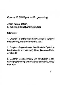
For example, consider the graph shown here. A TSP tour in the graph is 1-2-4-3-1. The cost of the tour is 10+25+30+15 which is 80.
Naï Na ïve Solution
Consider city 1 as the starting and ending point. Generate all (n-1)! Permutations of cities. Calculate cost of every permutation and keep track of minimum cost permutation. Return the permutation with minimum cost. Time Complexity: O(n!)
Dynamic Programming
Let the given set of vertices be {1, 2, 3, 4,….n}. Let us consider 1 as starting and ending point of output. For every other vertex i (other than 1), we find the minimum cost path with 1 as the starting point, i as the ending point and all vertices appearing exactly once.
Let the cost of this path be cost(i), the cost of corresponding Cycle would be cost(i) + dist(i, 1) where dist(i, 1) is the distance from i to 1. Finally, we return the minimum of all [cost(i) + dist(i, 1)] values. This looks simple so far. Now the question is how to get cost(i)?
Dynamic Programming
To calculate cost(i) using Dynamic Programming, we need to have some recursive relation in terms of sub-problems. Let us define a term C(S, i) be the cost of the minimum cost path visiting each vertex in set S exactly once, starting at 1 and ending at i. We start with all subsets of size 2 and calculate C(S, i) for all subsets where S is the subset, then we calculate C(S, i) for all subsets S of size 3 and so on. Note that 1 must be present in every subset.
If size of S is 2, then S must be {1, i},
C(S, i) = dist(1, i)
Else if size of S is greater than 2 then
C(S, i) = min { C(S-{i}, j) + dis(j, i)} where j belongs to S, j != i and j != 1.
TSP Distance Matrix
g(2,Ø) = c21 = 1
g(3,ø) = c31 = 15
g(4,ø) = c41 = 6
k = 1, consider sets of 1 element: Set {2}: g(3,{2}) = c32 + g(2,ø) = c32 + c21 = 7 + 1 = 8
p(3,{2}) = 2 g(4,{2}) = c42 + g(2,ø) = c42 + c21 = 3 + 1 = 4
p(4,{2}) = 2 Set {3}: g(2,{3}) = c23 + g(3,ø) = c23 + c31 = 6 + 15 = 21 p(2,{3}) = 3 g(4,{3}) = c43 + g(3,ø) = c43 + c31 = 12 + 15 = 27
p(4,{3}) = 3 Set {4}: g(2,{4}) = c24 + g(4,ø) = c24 + c41 = 4 + 6 = 10 p(2,{4}) = 4 g(3,{4}) = c34 + g(4,ø) = c34 + c41 = 8 + 6 = 14 p(3,{4}) = 4
k = 2, consider sets of 2 elements:
Set {2,3}: g(4,{2,3}) = min {c42 + g(2,{3}), c43 + g(3,{2})} = min {3+21, 12+8}= min {24, 20}= 20 p(4,{2,3}) = 3
Set {2,4}: g(3,{2,4}) = min {c32 + g(2,{4}), c34 + g(4,{2})} = min {7+10, 8+4}= min {17, 12} = 12 p(3,{2,4}) = 4
Set {3,4}: g(2,{3,4}) = min {c23 + g(3,{4}), c24 + g(4,{3})} = min {6+14, 4+27}= min {20, 31}= 20 p(2,{3,4}) = 3
Length of an optimal tour: f = g(1,{2,3,4}) =min{c12 + g(2,{3,4}), c13 + g(3,{2,4}), c14 + g(4,{2,3}) } = min {2 + 20, 9 + 12, 10 + 20} = min {22, 21, 30} = 21
Successor of node Successor of node Successor of node Optimal TSP tour:
1: p(1,{2,3,4}) = 3 3: p(3, {2,4}) = 4 4: p(4, {2}) = 2 1—> 3 —> 4 —> 2 —>1
Worksheet No. 21