as an activation function in the hidden layer of a three-layered neural network;. (2) For a ... functions. Hornik et al. 6] applied Stone-Weierstrass theorem, using ...
Accepted for publication by IEEE Transactions on Neural Networks.
Universal Approximation to Nonlinear Operators by Neural Networks with Arbitrary Activation Functions and Its Application to Dynamical Systems
Tianping Chen and Robert Chen 1
2
Abstract The purpose of this paper is to investigate neural network capability systematically. The main results are: (1) Every Tauber-Wiener function is quali ed as an activation function in the hidden layer of a three-layered neural network; (2) For a continuous function to be a Tauber-Wiener function, the necessary and su�cient condition is that it is not a polynomial; (3) The capability of approximating nonlinear functionals de ned on some Banach space and nonlinear operators has been shown, which implies that (4) we can use neural network computation to approximate the output as a whole (not at a xed point) of a dynamical system. Key words: Approximation theory, neural networks, dynamical systems, compact set, functional, operator. The author is with the Department of Mathematics, Fudan University, Shanghai, P.R.China. The author was with the Department of Electrical Engineering, University of Notre Dame, Notre Dame, Indiana 46556, USA. He is now with VLSI Libraries, Inc., 1836 Cabrillo Ave., Santa Clara, CA 95050. 1 2
1 Introduction There have been many papers related to approximation to a continuous function of several variables. In 1987, Wieland and Leighton [1] dealt with the capability of networks consisting of one or two hidden layers. Miyake and Irie [2] obtained an integral representation formula with an integral kernel xed beforehand. This representation formula is a kind of integrals, which could be realized by a threelayered neural network. In 1989, several papers related to this topic appeared. They all claimed that a three-layered neural network with sigmoid units on the hidden layer can approximate continuous or other kinds of functions de ned on compact set in Rn. They used di�erent methods. Carrol and Dickinson [4] used inverse Radon transform. Cybenko [3] used Hahn-Banach theorem and Riesz representation theorem. Funahashi [5] approximated Irie and Miyake's integral representation by a nite sum, using a kernel which can be expressed as a di�erence of two sigmoidal functions. Hornik et al. [6] applied Stone-Weierstrass theorem, using trigonometric functions. However, in all these papers, sigmoidal functions must be assumed to be continuous or monotone. Recently [9], we pointed out that the boundedness of the sigmoidal function plays an essential role for its being an activation function in the hidden layer. In addition to sigmoidal functions, many other functions can be used as activation functions in the hidden layer. For example, Hornik [6] proved that any bounded nonconstant continuous function is quali ed to be an activation function. Mhaskar and Micchelli [11] showed that under some restriction on the amplitude of a continuous 2
function near in nity, any non-polynomial function is quali ed to be an activation function. It is clear that all the aforementioned works are concerned with approximation to a continuous function de ned on a compact set in Rn (a space of nite dimensions). However, in engineering problems such as computing the output of dynamic systems or designing neural system identi ers, we often encounter the problem of approximating nonlinear functionals de ned on some function space, even nonlinear operators from one function space (a space of in nite dimensions) to another function space (another space of in nite dimensions). In [10], Sandberg gave an interesting theorem on approximating nonlinear functionals by superposition and composition of several linear functionals and a continuous function of one variable. Yet, two problems remain open: 1. Can we give those linear functionals explicitly? 2. Can we approximate nonlinear operators rather than functionals? Problem 1 is essential in application, since otherwise we are not able to construct real networks. Problem 2 is important in computing dynamic systems, for a dynamic system is in fact an operator. In [12], we discussed in detail the problem of approximating nonlinear functionals de ned on some compact set in C [a; b] or Lp[a; b] and obtained some explicit results. However, the problem of neural network's capability in approximating nonlinear operators with its related application in computing the output as a whole of a dynamic system still remains open. Moreover, a uni ed and systematic treatment of neural network approximation to continuous functions, functionals and operators is much needed but nevertheless also remains to be an open problem. 3
Speci cally, it is quite natural to raise the following issues: (1) What is the characteristic property for a continuous function in the hidden layer of a neural network? (2) To give a neural network model to approximate nonlinear functionals de ned on some compact set in C (K ), where K is some compact set in some Banach space. (3) To give a neural network model, which can be used to approximate the output of some dynamic system as a whole (not merely at a special point, cf. [10][12]), thus to identify the dynamic system. In this paper, we systematically give strong results for these issues. The paper is organized as follows. In section 2, we review some de nitions and notations. In section 3, we show that the necessary and su�cient condition for a continuous function in S 0(R ) (tempered distributions in R ) to be a Tauber-Wiener 1
1
function (for de nitions, see section 2) is that it is not a polynomial; and any TauberWiener function can be used as an activation function, i.e., any non-polynomial continuous function in S 0(R ) is an activation function. What is more interesting is 1
that we show the approximation is equiuniform on any compact set in C (K ), which is crucial in discussing approximation to continuous operators by neural networks. In section 4, we show the capability of neural networks to approximate continuous functionals de ned on some compact set in C (K ), where K is a compact set in some Banach space; and through which we establish the capability of neural networks to approximate continuous operators from C (K ) to C (K ). The main results in section 1
2
4 has a direct application to computing output of dynamic systems thus identifying the systems, which is discussed in section 5. 4
2 Notations and De nitions De nition 1.
A function � : R ! R is called a sigmoidal function, if it 1
satis es
(
1
limx!?1 �(x) = 0 ; limx!1 �(x) = 1 :
De nition 2. If a function g : R ! R (continuous or discontinuous) satis es that all the linear combinations PNi cig(�ix + �i), �i 2 R, �i 2 R, ci 2 R, i = =1
1; 2; : : : ; N , are dense in every C [a; b], then g is called a Tauber-Wiener function, or simply (TW) function.
De nition 3. Suppose that X is a Banach space, V � X is called a compact set in X , if for every sequence fxng1n with all xn 2 V , there is a subsequence fxn g, which converges to some element x 2 V . =1
k
It is well known that if V � X is a compact set in X , then for any � > 0, there is a �-net N (�) = fx ; : : : ; xn � g, with all xi 2 V , i = 1; : : : ; n(�), i.e. for every x 2 X , 1
( )
there is some xi 2 N (�) such that kxi ? xkX < �. In the sequel, we will often use the following notations.
X : some Banach space with norm k � kX .
Rn: Euclidean space of dimension n. K : some compact set in a Banach space. C (K ): Banach space of all continuous functions de ned on K , with norm kf kC K = (
5
)
maxx2K jf (x)j. (TW): All the Tauber-Wiener functions.
S (Rn): Schwartz functions in tempted distribution theory, i.e. rapidly decreasing and in nitely di�erentiable functions. S 0(Rn): Tempered distributions, i.e. linear continuous functionals de ned on S (Rn). C 1(Rn): In nitely di�erentiable functions. Cc1(Rn): In nitely di�erentiable functions with compact support in Rn. Cp[?1; 1]n: All 2-periodic functions with period 2 with respect to every variable xi, i = 1; : : : ; n.
3 Characteristics of Activation Functions In this Section, we prove three theorems.
Theorem 1 Suppose that g is a continuous function, and g 2 S 0(R ), then g 2 1
(TW ), if and only if g is not a polynomial.
Theorem 2 If � is a bounded sigmoidal function, then � 2 (TW ). Theorem 3 Suppose that K is a compact set in Rn , U is a compact set in C (K ), g 2 (TW ), then for any � > 0, there exist a positive integer N , real numbers �i, 6
vectors !i 2 Rn, i = 1; : : : ; N , which are independent of f 2 C (K ) and constants
ci(f ), i = 1; : : : ; N depending on f , such that
jf (x) ?
N X i=1
ci(f )g(!i � x + �i)j < �
(1)
holds for all x 2 K and f 2 U . Moreover, each ci (f ) is a linear continuous functional de ned on U .
Remark 1. Theorem 3 shows that for a function (continuous or discontinuous) to be quali ed as an activation function, a su�cient condition is that it belongs to (TW ) class. Therefore, in order to prove that a neural network is capable of approximating any continuous function of n variables, all we need to do is to deal with the case n = 1, thus we have reduced the complexity of the problem in terms of its dimensionality. Moreover, by examining the approximated function f (x ; : : :; xn) = 1
f (x ; 0; : : :; 0) = f � (x ), where f �(x ) is a continuous function of one variable, it is straightforward to see that the condition is also a necessary one. 1
1
1
Remark 2. The equiuniform convergence property in Theorem 3 will play a crucial role in approximating nonlinear operators by neural networks.
Remark 3.
When a sigmoidal function is used as an activation in a neu-
ral network, Theorem 2 shows that the only necessary condition imposed on is its boundedness. In contrast, in almost all other papers ([1], [2], [3], [4], [5], [6], [7], [8]), sigmoidal functions must be assumed to be either continuous or monotone.
Remark 4. In [11], some result similar to Theorem 1 was obtained under more restrictions imposed on g, i.e., there are positive integer N and a constant CN , such 7
that j(1 + jxj)?N g(x)j � C for all x 2 R . This restriction is essential for [11], for 1
the proof in [11] depends heavily on a variation of Paley-Wiener Theorem. However, in Theorem 1, we only assume that g 2 C (R ) \ S 0(Rn), which is weaker than the 1
assumptions used in [11].
Proof of Theorem 1. We will prove by contradiction. If all the linear combina-
tions Pni cig(�i x + �i) are not dense in C [a; b], then Hahn-Banach extension theorem =1
and Riesz representation of linear continuous functionals show that there is a signed Borel measure d� with supp(d�) � [a; b] and
Z g(�x + �) d�(x) = 0 R
(2)
1
for all � 6= 0 and � 2 R . Take any w 2 S (R ), then 1
1
Z Z w(�) d� R g(�x + �) d�(x) = 0: R 1
(3)
1
Let �x + � = u and change order of integration, we have Z Z �) = 0 g(u) w(�) d�( u ? � R R which is equivalent to ^ (��)) = 0 g^(w^(�)d� 1
(4)
1
(5)
where g^ represents Fourier transform of g in the sense of tempered distribution, and (5) is also understood in the sense of distribution (see [13]). In order that the left c (�t) 2 S (R ). Since hand side of (5) makes sense, we have to show that w^ (t)d� 1
c (t) 2 C 1(R ) and for each supp(d�) � [a; b], it is straightforward to show that d� k = 1; 2; : : :, there is a constant ck such that k c (t)j � ck : j @t@ k d� (6) 1
8
c (t) 2 S (R ). Consequently, w^(t)d� 1
c (t) 2 C 1 (R ), hence there exists some t 6= 0 with some Since d� 6� 0 and d� 1
0
c (t) 6= 0 for all t 2 (t ?�; t +� ). Now, if t 6= 0, neighborhood (t ?�; t +�) such that d� 0
0
0
0
1
c (�t) 6= 0 for all t 2 (t ? � ; t + � ). Take any w^ 2 Cc1 (t ? � ; t + � ), let � = tt , then d� � � � � 0
1
1
1
0
c (�t) 2 S (R ), and by (5) then w^(t)=d�
2
0
2
1
c (��)) = 0 g^(w^ (�)) = g^( cw^ (�) d� d�(��)
(7)
Previous argument shows that for any xed point t�, there is a neighborhood [t� ? �; t� + �] such that g^(w^(�)) = 0 for all w^ with compact support [t� ? �; t� + �], i.e. supp(^g) � f0g. By the distribution theory, g^ is some linear combination of �-Dirac function and its derivatives, which is equivalent to that g is a polynomial. Theorem 1 is proved. Proof of Theorem 2 can be found in [9]. Here we only give a brief proof for the completeness of this paper.
Proof of Theorem 2. Without loss of generality, we can assume that [a; b] = [0; 1]. Since f is continuous on [?1; 1] for any � > 0, there is an integer M > 0, such that jf (x0) ? f (x00)j < �=4, provided that x0; x00 2 [?1; 1] and jx0 ? x00j < 1=M . Divide [?1; 1] into 2M equal segments, each has length of 1=M . Let
? 1 = x < x < : : : < x M = 0 < xM < : : : < x M = 1 0
1
and ti = (xi + xi ), t? = ?1 ? 1 2
+1
1
+1
From the assumption, there exists W > 0,
M.
2
(8)
2
1
such that if u > W , then j�(u) ? 1j < M ; if u < ?W , then j�(u)j < M . Let K > 0 1
1
2
9
2
be such that K �
1
M
2
> W . Construct N X
g(x) = f (?M )�(K (x ? t? )) + [f (xi) ? f (xi? )]�(K (x ? ti? )) 1
1
i=1
1
(9)
then we can prove
jg(x) ? f (x)j < �
for all x 2 [?1; 1]
(10)
Theorem 2 is thus proved. Prior to proving Theorem 3, we need to establish the following lemmas.
Lemma 1 Suppose that K is a compact set in Rn, f 2 C (K ), then there is a continuous function E (f ) 2 C (Rn), such that (1) f (x) = E (f )(x) for all x 2 K ; (2) supx2R jE (f )(x)j � supx2K jf (x)j; (3) there is a constant c such that n
sup jE (f )(x0) ? E (f )(x00)j � c sup jf (x0) ? f (x00)j 0 00
jx0 ?x00 j 0 such that jf (x0) ?
f (x00)j < � for all f 2 V , provided that x0, x00 2 K and kx0 ? x00kK < �. 10
Lemma 3 Suppose that K is a compact set in In = [0; 1]n, V is a compact set in C (K ), then V can be extended to a compact set in Cp[?1; 1]n. By Lemmas 1 and 2, V can be extended to be a compact set V in C [0; 1]n.
Proof.
1
Now, for every f 2 V , de ne an even extension of f as follows 1
f � (x ; : : :; xk ; : : : ; xn) = f (x ; : : :; ?xk ; : : : ; xn) 1
(12)
1
then U = ff � : f 2 V g is the required compact set in Cp[?1; 1]n. 1
Lemma 4 Suppose that U is a compact set in Cp[?1; 1], X B (f ; x) = (1 ? jmj )�c (f )ei�m�x 2
R
R
2
jmj�R
(13)
m
is the Bochner-Riesz means of Fourier series of f , where m = (m1; : : : ; mn), jmj2 = Pn jm j2, c (f ) are Fourier coe�cients of f , then for any � > 0, there is R > 0 i=1
i
m
such that
jBR(f ; x) ? f (x)j < �
(14)
for every f 2 U and x 2 [?1; 1]n, provided that � > (n ? 1)=2. Proof.
The proof of Lemma 4 can be found in [13].
Proof of Theorem 3. Without loss of generality, we can assume that K � [0; 1]n. By Lemma 3, we can assume that K = [?1; 1]n and U � Cp[?1; 1]n. By Lemma 4, for any � > 0, there exists R > 0, such that for any x = (x ; : : :; xn) 2 [?1; 1]n and f 2 U , there holds X j (1 ? jmj )�c (f �)exp(i�(m x + � � � + m x )) ? f �(x ; : : : ; x )j < � (15) 1
2
jmj�R
R
2
m1 ���mn
1 1
11
n n
1
n
2
By the de nition of the Fourier coe�cients and evenness of f �(x), we can rewrite (15) as
j
X jmj�R
dm ���m cos(�(m x + � � � + mnxn ) ? f �(x ; : : :; xn)j < 2� 1
n
1
1
(16)
1
where dm ���m are real numbers. It is obvious that for every x 2 [?1; 1]n, there is a 1
n
p
p
unique u 2 [? n�R; n�R], such that
u = �m � x = �(m x + : : : + mnxn ) :
(17)
1 1
p
p
where m = (m ; : : :; mn). Since cos(u) is a continuous function in [? n�R; n�R] 1
and g 2 (TW ), we can nd an integer M , real numbers sj , �j and �j , j = 1; : : : ; M , such that
M X
j sj g(�j u + �j ) ? cos(u)j < 2�L j p p holds uniformly for all u 2 [? n�R; n�R], where L = P =1
jmj�R jdm1 ;:::;mn j.
M X
j sj g(�j �(m � x) + �j ) ? cos(�m � x)j < 2�L j =1
(18) Thus (19)
holds for x 2 [?1; 1]n. Substituting (19) into (16), we conclude that there exist N ,
ci, �i 2 R, !i 2 Rn, i = 1; : : : ; N , such that
jf �(x) ?
N X i=1
ci(f �)f �(!i � x + �i)j < �
is true for all x 2 [?1; 1]n and g 2 U . Thus
jf (x) ?
N X i=1
ci(f )g(!i � x + �i)j < �
is true for all x 2 [0; 1]n and f 2 V . 12
(20)
It is obvious that for each xed m = (m ; : : :; mn), the Fourier coe�cient 1
Z1 ?1
���
Z1 ?1
e?i� m x (
���+mn xn )g (x
1 1+
1
; : : :; xn) dx � � � dxn 1
is a continuous functional de ned on U (and also a continuous functional de ned on
V ), and ci(f ), being a nite linear combination of the Fourier coe�cients of f �, is surely a continuous functional de ned on V . The proof of Theorem 3 is completed.
4 Approximation to Nonlinear Continuous Functionals and Maps In this section, we will discuss the problem of approximating nonlinear continuous functionals and operators by neural network computation. The main results are as follows.
Theorem 4 Suppose that g 2 (TW ), X is a Banach Space, K � X is a compact set, V is a compact set in C (K ), f is a continuous functional de ned on V , then for any � > 0, there are an positive integer N , m points x1; : : :; xm 2 K , and real constants ci , �i, �ij , i = 1; : : : ; N , j = 1; : : : ; m, such that
jf (u) ?
N X i=1
m X
cig( �ij u(xj ) + �i)j < �
(21)
j =1
holds for all u 2 V .
Theorem 5 Suppose that g 2 (TW ), X is a Banach Space, K � X , K � Rn are two compact sets in X and Rn respectively, V is a compact set in C (K ), G is a 1
2
1
13
nonlinear continuous operator, which maps V into C (K2 ), then for any � > 0, there are positive integers M , N , m, constants cki , �k , �ijk 2 R, points !k 2 Rn, xj 2 K1,
i = 1; : : : ; M , k = 1; : : : ; N , j = 1; : : : ; m, such that m X k ci g( �ijk u(xj ) + �ik )g(!k � y + �k )j < � jG(u)(y) ? j =1 k=1 i=1 N X M X
(22)
holds for all u 2 V and y 2 K2 .
Following lemmas are well known and will be used in the proof of Theorems 4 and 5.
Lemma 5 Let X be a Banach Space and K � X , then K is a compact set if and only if the following two conditions are satis ed simultaneously: (1) K is a closed set in X ; (2) for any � > 0, there is a �-net N (�) = fx1 ; : : :; xn(�)g, i.e. for any x 2 K , there constitute an xk 2 N (�) such that kx ? xk kX < �.
Lemma 6 If V � C (K ) is a compact set in C (K ), then it is uniformly bounded and equicontinuous, i.e. (1) There is A > 0 such that ku(x)kC K � A for all u 2 V and (2) for any � > 0, there is � > 0 such that ju(x0) ? u(x00)j < � for all u 2 V , provided that kx0 ? x00kX < �. (
)
Now pick a sequence � > � > � � � > �n ! 0, then we can nd another sequence 1
2
� > � > � � � > �n ! 0, such that jf (u) ? f (v)j < �k for all f 2 V , provided that u; v 2 V and ku ? vkC K < 2�k , for f is a continuous functional de ned on a compact set V . 1
2
(
)
14
By Lemma 6, we can also nd � > � > � � � �n ! 0 such that ju(x0) ? u(x00)j < �k 1
2
for all u 2 V , whenever x0; x00 2 K and kx0 ? x00kK < �k . By induction and rearrangement, we can nd a sequence fxig1i with each xi 2 K =1
and a sequence of positive integers n(� ) < n(� ) < : : : < n(�k ) ! 1, such that the 1
2
rst n(�k ) elements N (�k ) = fx ; : : : ; xn � g is an �k -net in K . 1
( k)
For each �k -net, de ne functions
T��k ;j (x) =
(
1 ? kx?�x k 0
if kx ? xj kX � �k otherwise
j k
k
(23)
and
T � (x) (24) T� ;j (x) = Pn �� ;j � T ( x ) j � ;j for j = 1; : : : ; n(�k ). It is easy to verify that fT� ;j (x)g is a partition of unity, i.e. k ( k) =1
k
k
k
0 � T� ;j (x) � 1
(25)
k
nX (�k ) j =1
T� ;j (x) = 0 k
T� ;j (x) � 1 k
(26)
if kx ? xj kX > �k :
(27)
For each u 2 V , de ne a function
u� (x) = k
nX (�k ) j =1
u(xj )T� ;j (x) k
(28)
and sets V� = fu� : u 2 V g and V � = V [ ([1k V� ). We then have the following k
k
=1
result.
Lemma 7 15
k
1. For each xed k, V�k is a compact set in a subspace of dimension n(�k ) in C (K ). 2. For every u 2 V , there holds
ku ? u� kC K < �k (
k
(29)
)
3. V � is a compact set in C (K ). Proof.
We will prove the three propositions individually as follows.
1. For a xed k, let u�i , i = 1; 2; : : : ; be a sequence in V� and u i be a sequence ( ) k
( )
k
in V , such that
u�i = ( ) k
nX (�k ) j =1
u i (xj )T� ;j (x) : ( )
(30)
k
Since V is a compact set, there is a subsequence u i (x), which converges to some u 2 V , then it is obvious that u�i (x) converges to u� (x) 2 V� , i.e. V� ( l)
( l) k
k
k
k
is a compact subset in C (K ). 2. By the de nition and the property of unity partition, we have
u(x) ? u� (x) = k
=
nX (�k ) j =1
[u(x) ? u(xj )]T� ;j (x) k
X
kx?xj kX ��k
[u(x) ? u(xj )]T� ;j (x) :
(31)
k
Consequently,
ku(x) ? u� (x)kX � �k k
nX (�k ) j =1
T� ;j (x) = �k k
for all u 2 V :
(32)
� i 1 3. Suppose fuig1 j is a sequence in V . If there is a subsequence fu gl of fuig1j with all ui 2 V , l = 1; : : : ; then by the fact that V is compact, there is l
=1
=1
l
16
=1
a subsequence of fui g1 l , which converges to some u 2 V . Otherwise, to each l
=1
ui, there corresponds a positive integer k(i) such that ui = v� . There are two possibilities: (i) We can nd in nite il and a xed k such that �k i = �k i = � � � = �k i = � � � = �k , i.e. ui 2 V� for all il. By proposition 1. of this lemma, Vn � is a compact set, there is a subsequence of fvni � g, which converges to some v 2 Vn � , i.e. there is a subsequence of fuig converging to v 2 Vn � . (ii) There are sequences i < i < : : : ! 1 and k(i ) < k(i ) < : : : ! 1 such that ui 2 Vn � . Let vi 2 V be such that k (i)
0
( l)
l
0
( 1)
( 2)
k0
( k0 )
( k (i) )
( k0 )
( k0 )
1
l
( k (i ) ) l
2
1
2
l
uil (x) =
n(�X k (il ) ) j =1
vi (xj )T� l
k (il );j
(x) :
(33)
Since V i 2 V and V is compact, we see that there is a subsequence of fvi g1l , l
l
=1
which converges to some v 2 V . By the proposition 2. of this lemma, the corresponding subsequence of fui g1l also converges to v. Thus the compactness of V � is proved. l
=1
Proof of Theorem 4. By Tietze Extension Theorem, we can de ne a continuous functional on V � such that
f �(x) = f (x)
if x 2 V
(34)
Because f � is a continuous functional de ned on the compact set V �, therefore for any � > 0, we can nd a � > 0 such that jf �(u) ? f � (v)j < �=2 provided that u; v 2 V � and ku ? vkC K < �. (
)
Let k be xed such that �k < �, then by (29) for every u 2 V ,
ku ? u� kX < �k k
17
(35)
which implies
jf �(u) ? f �(u� )j < �=2
(36)
k
for all u 2 V . By proposition 1. of Lemma 7, we see that f � (u� ) is a continuous functional k
de ned on the compact set V� in Rn � . By Theorem 3, we can nd N , ci, �ij , �i, ( k)
k
i = 1; : : : ; N , j = 1; : : :; n(�k ), such that
jf �(u� ) ? k
N X i=1
cig(
nX (�k ) j =1
�ij u(xj ) + �i)j < �=2 :
(37)
Combining it with (36), we conclude that
jf (u) ?
N X i=1
m X
cig( �ij u(xj ) + �i)j < �
(38)
j =1
where m = n(�k ). Thus, Theorem 4 is proved.
Proof of Theorem 5.
From the assumption that G is a continuous operator which maps a compact set V in C (K ) into C (K ), it is straightforward to prove that 1
2
the range G(V ) = fG(u) : u 2 V g is also a compact set in C (K ). By Theorem 3, 2
for any � > 0, there are a positive integer N , real numbers ck (G(u)) and �k , vectors
!k 2 Rn, k = 1; : : : ; N , such that
jG(u)(y) ?
N X k=1
ck (G(u))g(!k � y + �k )j < �=2
(39)
holds for all y 2 K and u 2 V . 2
Since G is a continuous operator, combining with the last proposition of Theorem 3, we conclude that for each k = 1; : : : ; N , ck (G(u)) is a continuous functional de ned 18
on V . Repeatedly applying Theorem 4, for each k = 1; : : : ; N , we can nd positive integers Nk , mk , constants cki , �ijk , �ik 2 R and xj 2 K , i = 1; : : : ; Nk , j = 1; : : : ; mk, 1
such that
Nk X
mk X k jck (G(u)) ? ci g( �ijk u(xj ) + �ik )j < i=1 j =1
holds for all k = 1; : : :; N and u 2 V , where
L=
N X
� 2L
sup jg(!k � y + �k )j :
k=1 y2K2
(40)
(41)
Substituting (40) into (39), we obtain that
jG(u)(y) ?
Nk N X X k=1 i=1
mk X
cki g( �ijk u(xj ) + �ik )g(!k � y + �k )j < � j =1
(42)
holds for all u 2 V and y 2 K . 2
Let M = maxk fNk g, m = maxk fmk g and for all Nk < i � M , let cki = 0. For all mk < j � m, let �ijk = 0. Thus (42) can be rewritten as
jG(u)(y) ?
N X M X k=1 i=1
m X
cki g( �ijk u(xj ) + �ik )g(!k � y + �k )j < � j =1
(43)
holds for all u 2 V and y 2 K . This completes the proof of Theorem 5. 2
A graphical representation of Theorem 5 is shown in Fig. 1.
5 Application to Nonlinear Dynamical Systems In [12], we discussed the problem of approximating the output of a dynamical system at a xed point (or time) by neural networks. As a direct application of Theorem 5, we can use neural networks to approximate the output as a whole of a 19
nonlinear dynamical system. Indeed, built upon the several keystone theorems proved earlier in Section 4, our result on this topic follows naturally. The signi cance of the previous results lies in that we can use neural networks to identify a system (linear or nonlinear). The procedure is as follows: Let a system be V = KU , where U is the input, V is the output and K is the system to be identi ed. Suppose that according to some prior knowledge or experiments, we know several input-output relationships V = KU ; : : : ; Vn = KUn . Generally, they can be 1
1
expressed by discrete data sets fus(xj ); s = 1; : : : ; n; j = 1; : : : ; mg, fvs(yl); s = 1; : : : ; n; j = 1; : : : ; Lg. Using these data, and by Theorem 5, we can construct a functional
E=
m X k Ci g( �i;jk us(xj ) + �ik )g(!k � yl + �k )j2 jVs (yl) ? j =1 k=1 i=1 l=1 s=1 N X M X
L X n X
(44)
Parameters Cik , �i;jk , �ik , !k , � can be determined by minimizing E (for example, by using back-propagation algorithm). Then the equation m X k Ci g( �i;jk u(xj ) + �ik )g(!k � y + �k ) v(y) = j =1 k=1 i=1 N X M X
(45)
can be viewed as an approximant of V (y) = (KU )(y), and so identi es the system
K. If the system is linear, then E , V (y) can be simpli ed as
E=
n L X X l=1 s=1
jVs(yl) ?
m M X N X X k=1 i=1 j =1
20
�i;jk u(xj )g(!k � yl + �k )j
2
(46)
v(y) =
m N X M X X k=1 i=1 j =1
�i;jk u(xj )g(!k � y + �k ):
(47)
The larger the values of n, L, m are, the better accuracy we will obtain for this approximation. Therefore, we have pointed to a way of constructing neural network models for identifying dynamic systems.
Acknowledgements. The authors wish to express their gratefulness to the reviewers for their valuable comments and suggestions on revising this paper.
6 Conclusion In this paper, the problem of approximating functions of several variables, functionals and nonlinear operators are thoroughly studied. The necessary and su�cient condition for a continuous function in S 0(R ) to be quali ed for an activation function is 1
given, which is a broad generalization of previous results ([1]- [8], especially [11]). It is also pointed out that to prove neural network approximation capability, one needs only to treat the one dimensional case. As applications, we show how to construct neural networks to approximate the output of a dynamical system as a whole, not merely at a xed point, thus show the capability of neural network in identifying dynamic systems. Moreover, we point out that using existing algorithms in literatures (for example, back-propagation algorithm), we can determine those parameters in the network, i.e. identify the system. 21
References [1] A. Wieland and R. Leighten, \Geometric Analysis of Neural Network Capacity," in IEEE First ICNN. 1, pp. 385-392 (1987). [2] B. Irie and S. Miyake, \Capacity of Three-layered Perceptrons," in IEEE ICNN 1, pp. 641-648, (1988). [3] G. Cybenko, \Approximation by Superpositions of a Sigmoidal Function," in Math. of Control, Signals and Systems, Vol. 2, No. 4, pp. 303-314 (1989). [4] S. M. Carroll and B. W. Dickinson, \Construction of Neural Nets using Radon Transform," in IJCNN Proc. I, pp. 607-611 (1989). [5] K. Funahashi, \On the Approximate Realization of Continuous Mappings by Neural Networks," Neural Networks, pp. 183-192, Vol. 2, (1989). [6] K. Hornik, M. Stinchcombe and H. White, \Multi-layer Feedforward Networks are Universal Approximators," Neural Networks, Vol. 2, pp. 359-366 (1989). [7] K. Hornik, \Approximation Capabilities of Multilayer Feedforward Networks," Neural Networks, Vol. 4, pp. 251-257 (1991). [8] V. Y. Kreinovich, \Arbitrary Nonlinearity is Su�cient to Represent All Functions by Neural Networks: a Theorem," Neural Networks, Vol. 4, pp. 381-383 (1991). [9] Tianping Chen, Hong Chen and Ruey-wen Liu, \A Constructive Proof of Cybenko's Approximation Theorem and Its Extensions," pp. 163 - 168 in Computing Science and Statistics (editors LePage and Page), Proc. of the 22nd Symposium on the Interface (East Lansing, Michigan, May 1990), Springer-Verlag, ISBN 0-387-97719-8. Also submitted for publication. [10] I. W. Sandberg, \Approximations for Nonlinear Functionals," IEEE Trans. on Circuits and Systems, Vol. 39, No. 1, pp. 65-67, Jan. (1992). 22
[11] H.N. Mhaskar and C.A. Micchelli, \Approximation by Superposition of Sigmoidal and Radial Basis Functions," Advances in Applied Mathematics, Vol. 13, pp. 350373, (1992). [12] Tianping Chen and Hong Chen, \Approximation to Continuous Functionals by Neural Networks with Application to Dynamical Systems," accepted by IEEE Trans. on Neural Networks, to appear. [13] E. M. Stein and G. Weiss, Introduction to Fourier Analysis on Euclidean Spaces, Princeton University Press, (1971). [14] E. M. Stein, Singular Integrals and Di�erentiability Properties of Functions, Princeton University Press, (1970). [15] J. Diedonne, Foundation of Modern Analysis, Academic Press : New York and London (1969), p. 142.
23
INPUT 2: y = [ y y . . . y ] 1 n 2
y1
y2
yn
. . . . . . . ω2 n
ωN
ω12
n
ω1 n
Σ
Σ
ζ2
g
Σ
ζN
. . . . . . .
g
g
Σ
.
. . . . . . .
x
OUTPUT : Approx. to G(u)(y)
x
.
ζ1
.
ω11
x
c11
g
Σ . . . . . . .
Σ
2
cM1
c1
g
g
. . . . . . . c1N
cM2 . . . . . . .
g
g
Σ cMN
. . . . . . .
g
. . . . . . . 1
θ1
Σ
. . . . . . .
1 ξ1m 1 ξ11
Σ
1 θM
θ21
Σ
. . . . . . .
Σ
2 θM
1 ξ12
N ξ M2
1
ξM1
u(x1)
N
θ1
u(x2)
. . . . . . .
Σ
. . . . . . .
Σ
N
θM
N
N ξ1m
ξ Mm
u(xm )
Sampling Device
INPUT 1: u(x)
Figure 1: A neural network architecture of approximation to nonlinear operator G(u)(y) 24