Unpaired Image-to-Image Translation using Cycle-Consistent ...

Unpaired Image-to-Image Translation using Cycle-Consistent Adversarial Networks Jun-Yan Zhu∗ Taesung Park∗ Phillip Isola Alexei A. Efros Berkeley AI Research (BAIR) laboratory, UC Berkeley

arXiv:1703.10593v1 [cs.CV] 30 Mar 2017

Monet

Photos

Zebras

Horses

Summer

Monet

photo

zebra

horse

summer

photo

Monet

horse

zebra

winter

Photograph

Monet

Van Gogh

Cezanne

Winter

winter

summer

Ukiyo-e

Figure 1: Given any two unordered image collections X and Y , our algorithm learns to automatically “translate” an image from one into the other and vice versa: (left) 1074 Monet paintings and 6753 landscape photos from Flickr; (center) 1177 zebras and 939 horses from ImageNet; (right) 1273 summer and 854 winter Yosemite photos from Flickr. Example application (bottom): using a collection of paintings of a famous artist, learn to render a user’s photograph into their style.

Abstract

1. Introduction

Image-to-image translation is a class of vision and graphics problems where the goal is to learn the mapping between an input image and an output image using a training set of aligned image pairs. However, for many tasks, paired training data will not be available. We present an approach for learning to translate an image from a source domain X to a target domain Y in the absence of paired examples. Our goal is to learn a mapping G : X → Y such that the distribution of images from G(X) is indistinguishable from the distribution Y using an adversarial loss. Because this mapping is highly under-constrained, we couple it with an inverse mapping F : Y → X and introduce a cycle consistency loss to push F (G(X)) ≈ X (and vice versa). Qualitative results are presented on several tasks where paired training data does not exist, including collection style transfer, object transfiguration, season transfer, and photo enhancement, etc. Quantitative comparisons against several prior methods demonstrate the superiority of our approach.

What did Claude Monet see as he placed his easel by the bank of the Seine near Argenteuil on a lovely spring day in 1873 (Figure 1, top-left)? A color photograph, had it been invented, may have documented a crisp blue sky and a glassy river reflecting it. Monet conveyed his impression of this same scene through wispy brush strokes and a bright palette. What if Monet had happened upon the little harbor in Cassis on a cool summer evening (Figure 1, bottom-left)? A brief stroll through a gallery of Monet paintings makes it easy to imagine how he would have rendered the scene: perhaps in pastel shades, with abrupt dabs of paint, and a somewhat flattened dynamic range. We can imagine all this despite never having seen a side by side example of a Monet painting next to a photo of the scene he painted. Instead we have knowledge of the set of Monet paintings and of the set of landscape photographs. * indicates equal contribution

1

Paired

n xi

n

o

Y

,

…

o

( )( ) Unpaired

X

…

…

n

, , ,

yi o

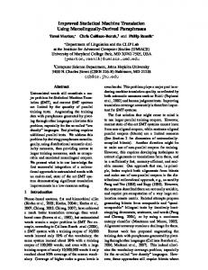
Figure 2: Paired training data (left) consists of training examples {xi , yi }N i=1 , where the yi that corresponds to each xi is given [18]. We instead consider unpaired training data (right), consisting of a source set {xi }N i=1 ∈ X and a target set {yj }M ∈ Y , with no information provided as to which j=1 xi matches which yj . We can reason about the stylistic differences between these two sets, and thereby imagine what a scene might look like if we were to “translate” it from one set into the other. In this paper, we present a system that can learn to do the same: capturing special characteristics of one image collection and figuring out how these characteristics could be translated into the other image collection, all in the absence of any paired training examples. This problem can be more broadly described as imageto-image translation [18], converting an image from one representation of a given scene, x, to another, y, e.g., greyscale to color, image to semantic labels, edge-map to photograph. Years of research in computer vision, image processing, and graphics have produced powerful translation systems in the supervised setting, where example image pairs {x, y} are available, e.g., [8, 15, 18, 19, 23, 28, 40, 50, 52, 55] (Figure 2, left). However, obtaining paired training data can be difficult and expensive. For example, only a couple of datasets exist for tasks like semantic segmentation (e.g., [3]), and they are relatively small. Obtaining input-output pairs for graphics tasks like artistic stylization can be even more difficult since the desired output is highly complex, typically requiring artistic authoring. For many tasks, like object transfiguration (e.g., zebra→horse, Figure 1 top-middle), the desired output is not even welldefined. We therefore seek an algorithm that can learn to translate between domains without paired input-output examples (Figure 2, right). We assume there is some underlying relationship between the domains – for example, that they are two different renderings of the same underlying world – and seek to learn that relationship. Although we lack supervision in the form of paired examples, we can exploit supervision at the level of sets: we are given one set of images in

domain X and a different set in domain Y . We may train a mapping G : X → Y such that the output yˆ = G(x), x ∈ X, is indistinguishable from images y ∈ Y by an adversary trained to classify yˆ apart from y. In theory, this objective can induce an output distribution over yˆ that matches the empirical distribution pY (y) (in general, this requires that G be stochastic) [13]. The optimal G thereby translates the domain X to a domain Yˆ distributed identically to Y . However, such a translation does not guarantee that the individual inputs and outputs x and y are paired up in a meaningful way – there are infinitely many mappings G that will induce the same distribution over yˆ. Moreover, in practice, we have found it difficult to optimize the adversarial objective in isolation: standard procedures often lead to the well-known problem of mode collapse, where all input images map to the same output image, and the optimization fails to make progress [12]. These issues call for adding more structure to our objective. We therefore exploit the property that translation should be “cycle consistent”, in the sense that if we translate, e.g., a sentence from English to French, and then translate it back from French to English, we should arrive back at the original sentence. Mathematically, if we have a translator G : X → Y and another translator F : Y → X, then G and F should be inverses of each other, and both mappings should be bijections. We apply this structural assumption by training both the mapping G and F simultaneously, and adding a cycle consistency loss that encourages F (G(x)) ≈ x and G(F (y)) ≈ y. Combining this loss with adversarial losses on domains X and Y yields our full objective for unpaired image-to-image translation. We apply our method on a wide range of applications, including style transfer, object transfiguration, attribute transfer and photo enhancement. We also compare against previous approaches that rely either on hand-defined factorizations of style and content, or on shared embedding functions, and show that our method outperforms these baselines. Our code is available at https://github.com/ junyanz/CycleGAN.

2. Related work Generative Adversarial Networks (GANs) [13, 56] have achieved impressive results in image generation [4, 33], image editing [59], and representation learning [38]. Recent methods adopt the same idea for conditional image generation applications, such as text2image [35], image inpainting [32], and future prediction [31], as well as to other domains like videos [48] and 3D models [51]. The key to GANs’ success is the idea of an adversarial loss that forces the generated images to be, in principle, indistinguishable from real images. This is particularly powerful for image generation tasks, as this is exactly the objective that much of computer graphics aims to optimize. We adopt an ad-

G

G X

Y

X

DY (a)

Yˆ

ˆ X

cycle-consistency loss

X(

ˆ X

Y

F

F DX

G Yˆ

F Y

(b)

X

(

Y

cycle-consistency loss

(c)

Figure 3: (a) Our model contains two mapping functions G : X → Y and F : Y → X, and associated adversarial discriminators DY and DX . DY encourages G to translate X into outputs indistinguishable from domain Y , and vice versa for DX , F , and X. To further regularize the mappings, we introduce two “cycle consistency losses” that capture the intuition that if we translate from one domain to the other and back again we should arrive where we started: (b) forward cycle-consistency loss: x → G(x) → F (G(x)) ≈ x, and (c) backward cycle-consistency loss: y → F (y) → G(F (y)) ≈ y versarial loss to learn the mapping such that the translated image cannot be distinguished from images in the target domain. Image-to-Image Translation The idea of image-toimage translation goes back at least to Hertzmann et al.’s Image Analogies [15], which employs a nonparametric texture model [7] from a single input-output training image pair. More recent approaches use a dataset of input-output examples to learn a parametric translation function using CNNs [28]. Our approach builds on the “pix2pix” framework of Isola et al. [18], which uses a conditional generative adversarial network [13] to learn a mapping from input to output images. Similar ideas have been applied to various tasks such as generating photographs from sketches [39] or from attribute and semantic layouts [20]. However, unlike these prior works, we learn the mapping without paired training examples. Unpaired Image-to-Image Translation Several other methods also tackle the unpaired setting, where the goal is to relate two data domains, X and Y . Rosales et al. [36] propose a Bayesian framework that includes a prior based on a patch-based Markov random field computed from a source image, and a likelihood term obtained from multiple style images. More recently, CoupledGANs [27] and cross-modal scene networks [1] use a weight-sharing strategy to learn a common representation across domains. Concurrent to our method, Liu et al. [26] extends this framework with a combination of variational autoencoders [22] and generative adversarial networks. Another line of concurrent work [41, 44, 2] encourages the input and output to share certain “content” features even though they may differ in “style“. They also use adversarial networks, with additional terms to enforce the output to be close to the input in a pre-defined metric space, such as class label space [2], image pixel space [41], and image feature space [44]. Unlike the above approaches, our formulation does not rely on any task-specific, pre-defined similarity function be-

tween the input and output, nor do we assume that the input and output have to lie in the same low-dimensional embedding space. This makes our method a general-purpose solution for many vision and graphics tasks. We directly compare against several prior approaches in Section 5.1. Neural Style Transfer [10, 19, 46, 9] is another way to perform image-to-image translation, which synthesizes a novel image by combining the content of one image with the style of another image (typically a painting) by matching the Gram matrix statistics of pre-trained deep features. Our main focus, on the other hand, is learning the mapping between two domains, rather than between two specific images, by trying to capture correspondences between higher-level appearance structures. Therefore, our method can be applied to other tasks, such as painting→ photo, object transfiguration, etc. where single sample transfer methods do not perform well. Cycle Consistency The idea of using transitivity as a way to regularize structured data has a long history. In visual tracking, enforcing simple forward-backward consistency has been a standard trick for decades [43]. More recently, higher-order cycle consistency has been used in structure from motion [54], 3D shape matching [17], cosegmentation [49], dense semantic alignment [57, 58], and depth estimation [11]. Of these, Zhou et al. [58] and Godard et al. [11] are most similar to our work, as they use a cycle consistency loss as a way of using transitivity to supervise CNN training. In this work, we are introducing a similar loss to push G and F to be consistent with each other.

3. Formulation Our goal is to learn mapping functions between two domains X and Y given training samples {xi }N i=1 ∈ X and {yj }M ∈ Y . As illustrated in Figure 3 (a), our model inj=1 cludes two mappings G : X → Y and F : Y → X. In addition, we introduce two adversarial discriminators DX and DY , where DX aims to distinguish between images

Input 𝑥

Generated image 𝐺(𝑥) Reconstruction F(𝐺 𝑥 )

3.2. Cycle Consistency Loss Adversarial training can, in theory, learn mappings G and F that produce outputs identically distributed as target domains Y and X respectively (strictly speaking, this requires G and F to be stochastic functions) [12]. However, with large enough capacity, a network can map the same set of input images to any random permutation of images in the target domain, where any of the learned mappings can induce an output distribution that matches the target distribution. Thus, an adversarial loss alone cannot guarantee that the learned function can map an individual input xi to a desired output yi . To further reduce the space of possible mapping functions, we argue that the learned mapping functions should be cycle-consistent: as shown in Figure 3 (b), for each image x from domain X, the image translation cycle should be able to bring x back to the original image, i.e. x → G(x) → F (G(x)) ≈ x. We call this forward cycle consistency. Similarly, as illustrated in Figure 3 (c), for each image y from domain Y , G and F should also satisfy backward cycle consistency: y → F (y) → G(F (y)) ≈ y. We can incentivize this behavior using a cycle consistency loss:

Figure 4: The reconstructed images F (G(x)) from various experiments. From top to bottom: photo↔Cezanne, horses↔zebras, winter→summer Yosemite, aerial maps↔maps on Google Maps. {x} and translated images {F (y)}; in the same way, DY aims to discriminate between {y} and {G(x)}. Our objective contains two terms: an adversarial loss [13] for matching the distribution of generated images to the data distribution in the target domain; and a cycle consistency loss to prevent the learned mappings G and F from contradicting each other.

3.1. Adversarial Loss We apply adversarial losses [13] to both mapping functions. For the mapping function G : X → Y and its discriminator DY , we express the objective as: LGAN (G, DY , X, Y ) =Ey∼pdata (y) [log DY (y)] +Ex∼pdata (x) [log(1 − DY (G(x))], (1) where G tries to generate images G(x) that look similar to images from domain Y , while DY aims to distinguish between translated samples G(x) and real samples y. G tries to minimize this objective against an adversarial D that tries to maximize it, i.e. G∗ = arg minG maxDY LGAN (G, DY , X, Y ). We introduce a similar adversarial loss for the mapping function F : Y → X and its discriminator DX as well: i.e. F ∗ = arg minF maxDX LGAN (F, DX , Y, X).

Lcyc (G, F ) =Ex∼pdata (x) [kF (G(x)) − xk1 ] +Ey∼pdata (y) [kG(F (y)) − yk1 ].

(2)

In preliminary experiments, we also tried replacing the L1 norm in this loss with an adversarial loss between F (G(x)) and x, and between G(F (y)) and y, but did not observe improved performance. The behavior induced by the cycle consistency loss can be observed in Figure 4: the reconstructed images F (G(x)) end up matching closely to the input images x.

3.3. Full Objective Our full objective is: L(G, F, DX , DY ) =LGAN (G, DY , X, Y ) + LGAN (F, DX , Y, X) + λLcyc (G, F ),

(3)

where λ controls the relative importance of the two objectives. We aim to solve: G∗ , F ∗ = arg min max L(G, F, DX , DY ). F,G Dx ,DY

(4)

Notice that our model can be viewed as training two “autoencoders” [16]: we learn one autoencoder F ◦ G : X → X jointly with another G ◦ F : Y → Y . However, these autoencoders each have special internal structure: they map an image to itself via an intermediate representation that is a translation of the image into another domain. Such a

setup can also be seen as a special case of “adversarial autoencoders” [29], which use an adversarial loss to train the bottleneck layer of an autoencoder to match an arbitrary target distribution. In our case, the target distribution for the X → X autoencoder is that of domain Y . In Section 5.1.4, we compare our full method against the adversarial loss LGAN alone and the cycle consistency loss alone Lcyc , and empirically show that both objectives play critical roles in arriving at high-quality results. We also evaluate our method with either only forward cycle loss or only backward cycle loss, and show that a single cycle is not be sufficient to regularize the training for this underconstrained problem.

see more datasets and training details in the appendix (Section 7).

5. Results We first compare our approach against recent methods for unpaired image-to-image translation on paired datasets where ground truth input-output pairs are available for evaluation. We then study the importance of both the adversarial loss and the cycle consistency loss, and compare our full method against several variants. Finally, we demonstrate the generality of our algorithm on a wide range of applications where paired data does not exist. For brevity, we refer to our method as CycleGAN.

4. Implementation Network Architecture We adapt the architecture for our generative networks from Johnson et al. [19] who have shown impressive results for neural style transfer and superresolution. This network contains two stride-2 convolutions, several residual blocks [14], and two fractionallystrided convolutions with stride 12 . We use 6 blocks for 128 × 128 images, and 9 blocks for 256 × 256 and higherresolution training images. Similar to Johnson et al. [19], we use instance normalization [47]. For the discriminator networks we use 70×70 PatchGANs [18, 25, 24], which try to classify whether 70 × 70 overlapping image patches are real or fake. Such a patch-level discriminator architecture has fewer parameters than a full-image discriminator, and can be applied to arbitrarily-sized images in a fully convolutional fashion. Training details We apply two techniques from prior works to stabilize our model training procedure. First, for LGAN (Equation 1), we replace the negative log likelihood objective by a least square loss [30]. This loss performs more stably during training and generates higher quality results. Equation 1 then becomes: LLSGAN (G, DY , X, Y ) =Ey∼pdata (y) [(DY (y) − 1)2 ] +Ex∼pdata (x) [DY (G(x))2 ],

(5)

Second, to reduce model oscillation [12], we follow Shrivastava et al’s strategy [41] and update discriminators DX and DY using a history of generated images rather than the ones produced by the latest generative networks. We keep an image buffer that stores the 50 previously generated images. For all the experiments, we set λ = 10 in Equation 3. We use the Adam solver [21] with a batch size of 1. All networks were trained from scratch, and trained with learning rate of 0.0002 for the first 100 epochs and a linearly decaying rate that goes to zero over the next 100 epochs. Please

5.1. Quantitative Evaluation Using the same evaluation datasets and metrics as “pix2pix” [18], we quantitatively test our method on the tasks of semantic labels↔photo on the Cityscapes dataset[3], and map↔aerial photo on data scraped from Google Maps. 5.1.1

Metrics

AMT perceptual studies On the maps↔photos task, we run “real vs fake” perceptual studies on Amazon Mechanical Turk (AMT) to assess the realism of our outputs. We follow the maps↔photos perceptual study protocol from [18], except we only gather data from 25 participants per algorithm we tested. Participants were shown a sequence of pairs of images, one a real photo or map and one fake (generated by our algorithm or a baseline), and asked to click on the image they thought was real. The first 10 trials of each session were practice and feedback was given as to whether the participant’s response was correct or incorrect. The remaining 40 trials were used to assess the rate at which each algorithm fooled participants. Each session only tested a single algorithm, and participants were only allowed to complete a single session. Note that the numbers we report here are not directly comparable to those in [18] as our ground truth images were processed slightly differently and the participant pool we tested may be differently distributed from those tested in [18] (due to running the experiment at a different date and time). Therefore, our numbers should only be used to compare our current method against the baselines (which were run under identical conditions), rather than against [18]. FCN score Although perceptual studies may be the gold standard for assessing graphical realism, we also seek an automatic quantitative measure that does not require human experiments. For this we adopt the “FCN score” from [18], and use it to evaluate the Cityscapes labels→photo task.

Input

BiGAN

CoGAN

CycleGAN

pix2pix

Ground truth

Figure 5: Different methods for mapping labels↔photos trained on cityscapes. From left to right: input, BiGAN [5, 6], CoupledGAN [27], CycleGAN (ours), pix2pix [18] trained on paired data, and ground truth. Input

BiGAN

CoGAN

CycleGAN

pix2pix

Ground truth

5.1.2

Baselines

CoGAN [27] This method learns one GAN generator for domain X and one for domain Y . The two generators share weights on their first few layers, which encourages them to learn a shared latent representation, with the subsequent unshared layers rendering the representation into the specific styles of X and Y . Translation from X to Y can be achieved by finding a latent representation that generates image X and then instead rendering this latent representation into style Y .

Figure 6: Different methods for mapping aerial photos↔maps on Google Maps. From left to right: input, BiGAN [5, 6], CoupledGAN [27], CycleGAN (ours), pix2pix [18] trained on paired data, and ground truth.

The FCN metric evaluates how interpretable the generated photos are according to an off-the-shelf semantic segmentation algorithm (the fully-convolutional network, FCN, from [28]). The FCN predicts a label map for a generated photo. This label map can then be compared against the input ground truth labels using standard semantic segmentation metrics described below. The intuition is that if we generate a photo from a label map of “car on road”, then we have succeeded if the FCN applied to the generated photo detects “car on road”.

Semantic segmentation metrics To evaluate the performance of photo→labels, we use the standard metrics from the Cityscapes benchmark, including per-pixel accuracy, per-class accuracy, and mean class Intersection-Over-Union (Class IOU) [3].

Pixel loss + GAN [41] Like our method, Shrivastava et al.[41] uses an adversarial loss to train a translation from X to Y . Whereas we regularize the mapping with a cycleconsistency loss, Shrivastava et al.[41] regularizes via the term kX − Yˆ k1 , which encourages the translation to be near an identity mapping. Feature loss + GAN We also test a variant of [41] where the L1 loss is computed over deep image features (VGG-16 relu4 2 [42]), rather than over RGB pixel values. Computing distances in deep feature space, like this, is also sometimes referred to as using a “perceptual loss” [19]. BiGAN [6, 5] Unconditional GANs [13] learn a generator G : Z → X, that maps random noise Z to images X. The BiGAN [6] and ALI [5] frameworks propose to also learn the inverse mapping function F : X → Z, which projects a generated image x back to a low-dimensional latent code z. Though originally designed for mapping a latent vector z to an image x, we implemented the same objective for mapping a source image x to a target image y. pix2pix [18] We also compare against pix2pix [18], which is trained on paired data, to see how close we can

Loss CoGAN [27] BiGAN [6, 5] Pixel loss + GAN [41] Feature loss + GAN CycleGAN (ours)

Map → Photo % Turkers labeled real 0.6% ± 0.5% 2.1% ± 1.0% 0.7% ± 0.5% 1.2% ± 0.6% 26.8% ± 2.8%

Photo → Map % Turkers labeled real 0.9% ± 0.5% 1.9% ± 0.9% 2.6% ± 1.1% 0.3% ± 0.2% 23.2% ± 3.4%

Table 1: AMT “real vs fake” test on maps↔aerial photos. Loss CoGAN [27] BiGAN [6, 5] Pixel loss + GAN [41] Feature loss + GAN CycleGAN (ours) pix2pix [18]

Per-pixel acc. 0.40 0.19 0.20 0.07 0.52 0.71

Per-class acc. 0.10 0.06 0.10 0.04 0.17 0.25

Class IOU 0.06 0.02 0.0 0.01 0.11 0.18

Table 2: FCN-scores for different methods, evaluated on Cityscapes labels→photos. get to this “upper bound” without using any paired training data. For fair comparison, we implement all the baselines, except the CoupledGAN [27], using the same architecture and implementation details as our method. CoupledGAN builds on generators that produce images from a shared latent representation, which is incompatible with our imageto-image architecture. We use the public implementation of this method instead 1 . 5.1.3

Comparison against baselines

As can be seen in Figure 5 and Figure 6, we were unable to achieve compelling results with any of the baselines. Our method, on the other hand, is able to produce translations that are often of similar quality to the fully supervised pix2pix. We exclude pixel loss + GAN and feature loss + GAN in the figures, as both of the methods fail to produce results at all close to the target domain (full results can be viewed at https://junyanz.github. io/CycleGAN/). Table 1 reports performance on the AMT perceptual realism task. Here, we see that our method can fool participants on around a quarter of trials, in both the map→photo direction and the photo→map direction. All baselines almost never fooled participants. Table 2 assesses the performance of the labels→photo task on the Cityscapes and Table 3 assesses the opposite mapping (photos→labels). In both cases, our method again outperforms the baselines. 5.1.4

Analysis of the loss function

In Table 4 and Table 5, we compare against ablations of our full loss. Removing the GAN loss substantially degrades results, as does removing the cycle-consistency 1 https://github.com/mingyuliutw/CoGAN

Loss CoGAN [27] BiGAN [6, 5] Pixel loss + GAN [41] Feature loss + GAN CycleGAN (ours) pix2pix [18]

Per-pixel acc. 0.45 0.41 0.47 0.50 0.58 0.85

Per-class acc. 0.11 0.13 0.11 0.10 0.22 0.40

Class IOU 0.08 0.07 0.07 0.06 0.16 0.32

Table 3: Classification performance of photo→labels for different methods on cityscapes. Loss Cycle alone GAN alone GAN + forward cycle GAN + backward cycle CycleGAN (ours)

Per-pixel acc. 0.22 0.52 0.55 0.41 0.52

Per-class acc. 0.07 0.11 0.18 0.14 0.17

Class IOU 0.02 0.08 0.13 0.06 0.11

Table 4: Ablation study: FCN-scores for different variants of our method, evaluated on Cityscapes labels→photos. Loss Cycle alone GAN alone GAN + forward cycle GAN + backward cycle CycleGAN (ours)

Per-pixel acc. 0.10 0.53 0.49 0.01 0.58

Per-class acc. 0.05 0.11 0.11 0.06 0.22

Class IOU 0.02 0.07 0.07 0.01 0.16

Table 5: Ablation study: classification performance of photos→labels for different losses, evaluated on Cityscapes. loss. We therefore conclude that both terms are critical to our results. We also evaluate our method with the cycle loss in only one direction: GAN+forward cycle loss Ex∼pdata (x) [kF (G(x)) − xk1 ], or GAN+backward cycle loss Ey∼pdata (y) [kG(F (y))−yk1 ] (Equation 2) and find that it often incurs training instability and causes mode collapse, especially for the direction of the mapping that was removed. Figure 7 shows several qualitative examples. 5.1.5

Image reconstruction quality

In Figure 4, we show a few random samples of the reconstructed images F (G(x)) or G(F (y)). We observed that the reconstructed images were very close to the original inputs x and y, at both training and testing time, even in cases where one domain represents significantly more diverse information, such as map↔aerial photos. 5.1.6

Additional results on paired datasets

Figure 8 shows some example results on other paired datasets used in “pix2pix” [18], such as architectural labels↔photos from the CMP Facade Database [34], and edges↔shoes from the UT Zappos50K dataset [53]. The image quality of our results is close to those produced by the fully supervised pix2pix while our method learns the mapping without input-output supervision.

Input

Cycle alone

GAN alone

GAN+forward

GAN+backward Ours+Identity loss CycleGAN (ours)

Ground truth

Figure 7: Different variants of our method for mapping labels↔photos trained on cityscapes. From left to right: input, cycleconsistency loss alone, adversarial loss alone, GAN + forward cycle-consistency loss (F (G(x)) ≈ x), GAN + backward cycle-consistency loss (G(F (y)) ≈ y), CycleGAN (our full method), and ground truth. Both Cycle alone and GAN + backward fail to produce images similar to the target domain. GAN alone and GAN + forward suffer from mode collapse, producing identical label maps regardless of the input photo. Input

Output

Input

Output

Input

Output

label → facade

facade → label

edges → shoes

edges → shoes

Figure 8: Example results of CycleGAN on paired datasets used in “pix2pix” [18] such as architectural labels↔photos and edges↔shoes.

style transfer” [10], our method learns to mimic the style of an entire set of artworks, rather than transferring the style of a single selected piece of art. Therefore, we can learn to generate photos in the style of, e.g., Van Gogh, rather than just in the style of Starry Night. The size of the dataset for each artist/style was 526, 1073, 400, and 563 for Cezanne, Monet, Van Gogh, and Ukiyo-e. All artwork images were fetched from Wikiart. Object transfiguration (Figure 13) The model is trained to translate one object class from Imagenet [37] to another (each class contains around 1000 training images). Turmukhambetov et al.[45] proposes a subspace model to translate one object into another object of the same category, while our method focuses on object transfiguration between two visually similar categories. Season transfer (Figure 13) The model is trained on 854 winter photos and 1273 summer photos of Yosemite downloaded from Flickr.

5.2. Applications We demonstrate our method on several applications where unpaired training data does not exist. Please refer to Section 7 for more details about the datasets. We observe that translations on training data are often more appealing than those on test data, and full results of all applications on both training and test data can be viewed on our project website https://junyanz.github.io/ CycleGAN/. Collection style transfer (Figure 10 and Figure 11) We train the model on landscape photographs downloaded from Flickr and WikiArt. Note that unlike recent work on “neural

Photo generation from paintings (Figure 12) For painting→photo, we find that it is helpful to introduce an additional loss to encourage the mapping to preserve color composition between the input and output. In particular, we adopt the technique of Taigman et al. [44] and regularize the generator to be near an identity mapping when real samples of the target domain are provided as the input to the generator: i.e. Lidentity (G, F ) = Ey∼pdata (y) [kG(y) − yk1 ] + Ex∼pdata (x) [kF (x) − xk1 ]. Without Lidentity , the generator G and F are free to change the tint of input images when there is no need to. For example, when learning the mapping between Monet’s paintings and Flickr photographs, the generator often maps

Input

CycleGAN

CycleGAN+𝐿𝑖𝑑𝑒𝑛𝑡𝑖𝑡𝑦

an entire collection, we compute the average Gram Matrix across the target domain, and use this matrix to transfer the “average style” using [10]. Figure 16 demonstrates similar comparisons for other translation tasks. We observe that Gatys et al. [10] requires finding target style images that closely match the desired output, but still often fails to produce photo-realistic results, while our method succeeds to generate natural looking results, similar to the target domain.

6. Limitations and Discussion

Figure 9: The effect of the identity mapping loss on Monet→ Photo. From left to right: input paintings, CycleGAN without identity mapping loss, CycleGAN with identity mapping loss. The identity mapping loss helps preserve the color of the input paintings. paintings of daytime to photographs taken during sunset, because such a mapping may be equally valid under the adversarial loss and cycle consistency loss. The effect of this identity mapping loss are shown in Figure 9. In Figure 12, we show additional results translating Monet paintings to photographs. This figure and Figure 9 and show results on paintings that were included in the training set, whereas for all other experiments in the paper, we only evaluate and show test set results. Because the training set does not include paired data, coming up with a plausible translation for a training set painting is a nontrivial task. Indeed, since Monet is no longer able to create new paintings, generalization to unseen, “test set”, paintings is not a pressing problem. Photo enhancement (Figure 14) We show that our method can be used to generate photos with shallower depth of field. We train the model on flower photos downloaded from Flickr. The source domain consists of photos of flower taken by smartphones, which usually have deep DoF due to small aperture. The target contains photos taken with DSLRs with larger aperture. Our model successfully generates photos with shallower depth of field from the photos taken by smartphones. Comparison with Gatys et al. [10] In Figure 15, we compare our results with neural style transfer [10] on photo stylization. For each row, we first use two representative artworks as the style images for [10]. Our method, on the other hand, is able to produce photos in the style of entire collection. To compare against neural style transfer of

Although our method can achieve compelling results in many cases, the results are far from uniformly positive. Several typical failure cases are shown in Figure 17. On translation tasks that involve color and texture changes, like many of those reported above, the method often succeeds. We have also explored tasks that require geometric changes, with little success. For example, on the task of dog→cat transfiguration, the learned translation degenerates to making minimal changes to the input (Figure 17). Handling more varied and extreme transformations, especially geometric changes, is an important problem for future work. We also observe a lingering gap between the results achievable with paired training data and those achieved by our unpaired method. In some cases, this gap may be very hard – or even impossible,– to close: for example, our method sometimes permutes the labels for tree and building in the output of the photos→labels task. To resolve this ambiguity may require some form of weak semantic supervision. Integrating weak or semi-supervised data may lead to substantially more powerful translators, still at a fraction of the annotation cost of the fully-supervised systems. Nonetheless, in many cases completely unpaired data is plentifully available and should be made use of. This paper pushes the boundaries of what is possible in this “unsupervised” setting. Acknowledgments: We thank Aaron Hertzmann, Shiry Ginosar, Deepak Pathak, Bryan Russell, Eli Shechtman, Richard Zhang, and Tinghui Zhou for many helpful comments. This work was supported in part by NSF SMA1514512, a Google Research Award, Intel Corp, and hardware donations from NVIDIA. JYZ is supported by the Facebook Graduate Fellowship and TP is supported by the Samsung Scholarship. The photographs used in style transfer were taken by AE, mostly in France.

Input

Monet

Van Gogh

Cezanne

Ukiyo-e

Figure 10: Collection style transfer: we transfer input images into the artistic styles of Monet, Van Gogh, Cezanne, and Ukiyo-e. Please see our website for additional examples.

Input

Monet

Van Gogh

Cezanne

Ukiyo-e

Figure 11: Collection style transfer: we transfer input images into the artistic styles of Monet, Van Gogh, Cezanne, Ukiyo-e. Please see our website for additional examples.

Input

Output

Input

Output

Figure 12: Relatively successful results on mapping Monet paintings to photographs. Please see our website for additional examples.

Input

Output

Input

Output

Input

Output

horse → zebra

zebra → horse

winter Yosemite → summer Yosemite

summer Yosemite → winter Yosemite

apple → orange

orange → apple Figure 13: Our method applied to several translation problems. These images are selected as relatively successful results – please see our website for more comprehensive and random results. In the top two rows, we show results on object transfiguration between horses and zebras, trained on 939 images from the wild horse class and 1177 images from the zebra class in Imagenet [37]. The middle two rows show results on season transfer, trained on winter and summer photos of Yosemite from Flickr. In the bottom two rows, we train our method on 996 apple images and 1020 navel orange images from ImageNet.

Input

Output

Input

Output

Input

Output

Input

Output

Figure 14: Photo enhancement: mapping from a set of iPhone snaps to professional DSLR photographs, the system often learns to produce shallow focus. Here we show some of the most successful results in our test set – average performance is considerably worse. Please see our website for more comprehensive and random examples.

Input

Gatys et al. (image I)

Gatys et al. (image II)

Gatys et al. (collection)

CycleGAN

Photo → Van Gogh

Photo → Ukiyo-e

Photo → Cezanne

Figure 15: We compare our method with neural style transfer [10] on photo stylization. Left to right: input image, results from [10] using two different representative artworks as style images, results from [10] using the entire collection of the artist, and CycleGAN (ours).

Input

Gatys et al. (image I)

Gatys et al. (image II)

Gatys et al. (collection)

CycleGAN

apple → orange

horse → zebra

Monet → photo

Figure 16: We compare our method with neural style transfer [10] on various applications. From top to bottom: apple→orange, horse→zebra, and Monet→photo. Left to right: input image, results from [10] using two different images as style images, results from [10] using all the images from the target domain, and CycleGAN (ours).

Input

Output

apple → orange

dog → cat

photo → Ukiyo-e

Input

Output

zebra → horse

cat → dog

photo → Van Gogh

Input

Output

winter → summer

Monet → photo

iPhone photo → DSLR photo

Figure 17: Typical failure cases of our method. Please see our website for more comprehensive results.

References [1] Y. Aytar, L. Castrejon, C. Vondrick, H. Pirsiavash, and A. Torralba. Cross-modal scene networks. arXiv preprint arXiv:1610.09003, 2016. 3 [2] K. Bousmalis, N. Silberman, D. Dohan, D. Erhan, and D. Krishnan. Unsupervised pixel-level domain adaptation with generative adversarial networks. arXiv preprint arXiv:1612.05424, 2016. 3 [3] M. Cordts, M. Omran, S. Ramos, T. Rehfeld, M. Enzweiler, R. Benenson, U. Franke, S. Roth, and B. Schiele. The cityscapes dataset for semantic urban scene understanding. In CVPR, 2016. 2, 5, 6, 19 [4] E. L. Denton, S. Chintala, R. Fergus, et al. Deep generative image models using a laplacian pyramid of adversarial networks. In NIPS, pages 1486–1494, 2015. 2 [5] J. Donahue, P. Kr¨ahenb¨uhl, and T. Darrell. Adversarial feature learning. arXiv preprint arXiv:1605.09782, 2016. 6, 7 [6] V. Dumoulin, I. Belghazi, B. Poole, A. Lamb, M. Arjovsky, O. Mastropietro, and A. Courville. Adversarially learned inference. arXiv preprint arXiv:1606.00704, 2016. 6, 7 [7] A. A. Efros and T. K. Leung. Texture synthesis by non-parametric sampling. In ICCV, volume 2, pages 1033–1038. IEEE, 1999. 3 [8] D. Eigen and R. Fergus. Predicting depth, surface normals and semantic labels with a common multi-scale convolutional architecture. In ICCV, pages 2650– 2658, 2015. 2 [9] L. A. Gatys, M. Bethge, A. Hertzmann, and E. Shechtman. Preserving color in neural artistic style transfer. arXiv preprint arXiv:1606.05897, 2016. 3 [10] L. A. Gatys, A. S. Ecker, and M. Bethge. Image style transfer using convolutional neural networks. CVPR, 2016. 3, 8, 9, 14, 15 [11] C. Godard, O. Mac Aodha, and G. J. Brostow. Unsupervised monocular depth estimation with left-right consistency. arXiv preprint arXiv:1609.03677, 2016. 3 [12] I. Goodfellow. Nips 2016 tutorial: Generative adversarial networks. arXiv preprint arXiv:1701.00160, 2016. 2, 4, 5 [13] I. Goodfellow, J. Pouget-Abadie, M. Mirza, B. Xu, D. Warde-Farley, S. Ozair, A. Courville, and Y. Bengio. Generative adversarial nets. In NIPS, 2014. 2, 3, 4, 6 [14] K. He, X. Zhang, S. Ren, and J. Sun. Deep residual learning for image recognition. In CVPR, pages 770– 778, 2016. 5

[15] A. Hertzmann, C. E. Jacobs, N. Oliver, B. Curless, and D. H. Salesin. Image analogies. pages 327–340. ACM, 2001. 2, 3 [16] G. E. Hinton and R. R. Salakhutdinov. Reducing the dimensionality of data with neural networks. Science, 313(5786):504–507, 2006. 4 [17] Q.-X. Huang and L. Guibas. Consistent shape maps via semidefinite programming. In Computer Graphics Forum, volume 32, pages 177–186. Wiley Online Library, 2013. 3 [18] P. Isola, J.-Y. Zhu, T. Zhou, and A. A. Efros. Imageto-image translation with conditional adversarial networks. arXiv preprint arXiv:1611.07004, 2016. 2, 3, 5, 6, 7, 8, 19 [19] J. Johnson, A. Alahi, and L. Fei-Fei. Perceptual losses for real-time style transfer and super-resolution. In ECCV, pages 694–711. Springer, 2016. 2, 3, 5, 6, 19 [20] L. Karacan, Z. Akata, A. Erdem, and E. Erdem. Learning to generate images of outdoor scenes from attributes and semantic layouts. arXiv preprint arXiv:1612.00215, 2016. 3 [21] D. Kingma and J. Ba. Adam: A method for stochastic optimization. arXiv preprint arXiv:1412.6980, 2014. 5 [22] D. P. Kingma and M. Welling. Auto-encoding variational bayes. ICLR, 2014. 3 [23] P.-Y. Laffont, Z. Ren, X. Tao, C. Qian, and J. Hays. Transient attributes for high-level understanding and editing of outdoor scenes. ACM Transactions on Graphics (TOG), 33(4):149, 2014. 2 [24] C. Ledig, L. Theis, F. Husz´ar, J. Caballero, A. Cunningham, A. Acosta, A. Aitken, A. Tejani, J. Totz, Z. Wang, et al. Photo-realistic single image superresolution using a generative adversarial network. arXiv preprint arXiv:1609.04802, 2016. 5 [25] C. Li and M. Wand. Precomputed real-time texture synthesis with markovian generative adversarial networks. ECCV, 2016. 5 [26] M.-Y. Liu, T. Breuel, and J. Kautz. Unsupervised image-to-image translation networks. arXiv preprint arXiv:1703.00848, 2017. 3 [27] M.-Y. Liu and O. Tuzel. Coupled generative adversarial networks. In NIPS, pages 469–477, 2016. 3, 6, 7 [28] J. Long, E. Shelhamer, and T. Darrell. Fully convolutional networks for semantic segmentation. In CVPR, pages 3431–3440, 2015. 2, 3, 6 [29] A. Makhzani, J. Shlens, N. Jaitly, I. Goodfellow, and B. Frey. Adversarial autoencoders. arXiv preprint arXiv:1511.05644, 2015. 5

[30] X. Mao, Q. Li, H. Xie, R. Y. Lau, and Z. Wang. Multiclass generative adversarial networks with the l2 loss function. arXiv preprint arXiv:1611.04076, 2016. 5 [31] M. Mathieu, C. Couprie, and Y. LeCun. Deep multiscale video prediction beyond mean square error. ICLR, 2016. 2 [32] D. Pathak, P. Krahenbuhl, J. Donahue, T. Darrell, and A. A. Efros. Context encoders: Feature learning by inpainting. CVPR, 2016. 2 [33] A. Radford, L. Metz, and S. Chintala. Unsupervised representation learning with deep convolutional generative adversarial networks. arXiv preprint arXiv:1511.06434, 2015. 2 ˇ Radim Tyleˇcek. Spatial pattern templates for [34] R. S. recognition of objects with regular structure. In Proc. GCPR, Saarbrucken, Germany, 2013. 7, 19 [35] S. Reed, Z. Akata, X. Yan, L. Logeswaran, B. Schiele, and H. Lee. Generative adversarial text to image synthesis. arXiv preprint arXiv:1605.05396, 2016. 2 [36] R. Rosales, K. Achan, and B. J. Frey. Unsupervised image translation. In iccv, pages 472–478, 2003. 3 [37] O. Russakovsky, J. Deng, H. Su, J. Krause, S. Satheesh, S. Ma, Z. Huang, A. Karpathy, A. Khosla, M. Bernstein, et al. Imagenet large scale visual recognition challenge. IJCV, 115(3):211–252, 2015. 8, 13 [38] T. Salimans, I. Goodfellow, W. Zaremba, V. Cheung, A. Radford, and X. Chen. Improved techniques for training gans. arXiv preprint arXiv:1606.03498, 2016. 2

[45] D. Turmukhambetov, N. D. Campbell, S. J. Prince, and J. Kautz. Modeling object appearance using context-conditioned component analysis. In CVPR, pages 4156–4164, 2015. 8 [46] D. Ulyanov, V. Lebedev, A. Vedaldi, and V. Lempitsky. Texture networks: Feed-forward synthesis of textures and stylized images. In Int. Conf. on Machine Learning (ICML), 2016. 3 [47] D. Ulyanov, A. Vedaldi, and V. Lempitsky. Instance normalization: The missing ingredient for fast stylization. arXiv preprint arXiv:1607.08022, 2016. 5 [48] C. Vondrick, H. Pirsiavash, and A. Torralba. Generating videos with scene dynamics. In NIPS, pages 613– 621, 2016. 2 [49] F. Wang, Q. Huang, and L. J. Guibas. Image cosegmentation via consistent functional maps. In ICCV, pages 849–856, 2013. 3 [50] X. Wang and A. Gupta. Generative image modeling using style and structure adversarial networks. ECCV, 2016. 2 [51] J. Wu, C. Zhang, T. Xue, B. Freeman, and J. Tenenbaum. Learning a probabilistic latent space of object shapes via 3d generative-adversarial modeling. In NIPS, pages 82–90, 2016. 2 [52] S. Xie and Z. Tu. Holistically-nested edge detection. In ICCV, 2015. 2 [53] A. Yu and K. Grauman. Fine-grained visual comparisons with local learning. In CVPR, pages 192–199, 2014. 7, 19

[39] P. Sangkloy, J. Lu, C. Fang, F. Yu, and J. Hays. Scribbler: Controlling deep image synthesis with sketch and color. arXiv preprint arXiv:1612.00835, 2016. 3

[54] C. Zach, M. Klopschitz, and M. Pollefeys. Disambiguating visual relations using loop constraints. In CVPR, pages 1426–1433. IEEE, 2010. 3

[40] Y. Shih, S. Paris, F. Durand, and W. T. Freeman. Datadriven hallucination of different times of day from a single outdoor photo. ACM Transactions on Graphics (TOG), 32(6):200, 2013. 2

[55] R. Zhang, P. Isola, and A. A. Efros. Colorful image colorization. ECCV, 2016. 2

[41] A. Shrivastava, T. Pfister, O. Tuzel, J. Susskind, W. Wang, and R. Webb. Learning from simulated and unsupervised images through adversarial training. arXiv preprint arXiv:1612.07828, 2016. 3, 5, 6, 7 [42] K. Simonyan and A. Zisserman. Very deep convolutional networks for large-scale image recognition. arXiv preprint arXiv:1409.1556, 2014. 6 [43] N. Sundaram, T. Brox, and K. Keutzer. Dense point trajectories by gpu-accelerated large displacement optical flow. In ECCV, pages 438–451. Springer, 2010. 3 [44] Y. Taigman, A. Polyak, and L. Wolf. Unsupervised cross-domain image generation. arXiv preprint arXiv:1611.02200, 2016. 3, 8

[56] J. Zhao, M. Mathieu, and Y. LeCun. Energybased generative adversarial network. arXiv preprint arXiv:1609.03126, 2016. 2 [57] T. Zhou, Y. Jae Lee, S. X. Yu, and A. A. Efros. Flowweb: Joint image set alignment by weaving consistent, pixel-wise correspondences. In CVPR, pages 1191–1200, 2015. 3 [58] T. Zhou, P. Krahenbuhl, M. Aubry, Q. Huang, and A. A. Efros. Learning dense correspondence via 3dguided cycle consistency. In CVPR, pages 117–126, 2016. 3 [59] J.-Y. Zhu, P. Kr¨ahenb¨uhl, E. Shechtman, and A. A. Efros. Generative visual manipulation on the natural image manifold. In ECCV, 2016. 2

7. Appendix 7.1. Training details All networks (except Edges↔shoes) were trained from scratch, with learning rate of 0.0002 for the first 100 epochs and linearly decaying rate to zero for the next 100 epochs. Weights were initialized from a Gaussian distribution with mean 0 and standard deviation 0.02. Cityscapes label↔Photo 2975 training images from the Cityscapes training set [3] with image size 128 × 128. We used the Cityscapes val set for testing. Maps↔aerial photograph 1096 training images scraped from Google Maps [18] with image size 256 × 256. Images were sampled from in and around New York City. Data was then split into train and test about the median latitude of the sampling region (with a buffer region added to ensure that no training pixel appeared in the test set). Architectural facades labels↔photo 400 training images from [34]. Edges→shoes 50k training images from UT Zappos50K dataset [53]. The model was trained for 5 epochs with learning rate of 0.0002. Horse↔Zebra and Apple↔Orange The images for each class were downloaded from ImageNet using keywords wild horse, zebra, apple, and navel orange. The images were scaled to 256×256 pixels. The training set size of each class was horse: 939, zebra: 1177, apple: 996, orange: 1020. Summer↔Winter Yosemite The images were downloaded using Flickr API using the tag yosemite and the datetaken field. Black-and-white photos were pruned. The images were scaled to 256 × 256 pixels. The training size of each class was summer: 1273, winter: 854. Photo↔Art for style transfer The art images were downloaded from Wikiart.org by crawling. Some artworks that were sketches or too obscene were pruned by hand. The photos are downloaded from Flickr using the combination of tags landscape and landscapephotography. Blackand-white photos were pruned. The images were scaled to 256 × 256 pixels. The training set size of each class was Monet: 1074, Cezanne: 584, Van Gogh: 401, Ukiyo-e: 1433, Photographs: 6853. The Monet dataset was particularly pruned to include only landscape paintings, and Van Gogh included only his later works that represent his most recognizable artistic style.

Monet→Photo In order to achieve high resolution while conserving memory, random square crops of the rectangular images were used for training. To generate results, images of width 512 pixels with correct aspect ratio were passed to the generator network as input. The weight for the identity mapping loss was 0.5. Flower photo enhancement Flower images taken on iPhones were downloaded from Flickr by searching for the photos taken by Apple iPhone 5, 5s, or 6, with search text flower. DSLR images with shallow DoF were also downloaded from Flickr by search tag flower, dof. The images were scaled to width 360 pixels. The identity mapping loss of weight 0.5 was used. The training set size of the smartphone and DSLR dataset were 1813 and 3326, respectively.

7.2. Network architectures Code and models are available at https://github. com/junyanz/CycleGAN. Generator architectures We adapt our architectures from Johnson et al. [19]. We use 6 blocks for 128 × 128 training images, and 9 blocks for 256 × 256 or higherresolution training images. Below, we follow the naming convention used in the Johnson el al.’s Github repository2 Let c7s1-k denote a 7 × 7 Convolution-BatchNormReLU layer with k filters and stride 1. dk denotes a 3 × 3 Convolution-BatchNorm-ReLU layer with k filters, and stride 2. Reflection padding was used to reduce artifacts. Rk denotes a residual block that contains two 3 × 3 convolutional layers with the same number of filters on both layer. uk denotes a 3 × 3 fractional-strided-ConvolutionBatchNorm-ReLU layer with k filters, and stride 21 . The network with 6 blocks consists of: c7s1-32,d64,d128,R128,R128,R128, R128,R128,R128,u64,u32,c7s1-3 The network with 9 blocks consists of: c7s1-32,d64,d128,R128,R128,R128, R128,R128,R128,R128,R128,R128,u64,u32,c7s1-3 Discriminator architectures For discriminator networks, we use 70 × 70 PatchGAN [18]. Let Ck denote a 4 × 4 Convolution-BatchNorm-LeakyReLU layer with k filters and stride 2. After the last layer, we apply a convolution to produce a 1 dimensional output. We do not use BatchNorm for the first C64 layer. We use leaky ReLUs with slope 0.2. The discriminator architecture is: C64-C128-C256-C512

2 https://github.com/jcjohnson/ fast-neural-style.