Unraveling Multi-Dimensional Data using pDView Luigi Di Caro
Maria Luisa Sapino
K. Selçuk Candan
Universita’ di Torino Dip. di Informatica
Universita’ di Torino Dip. di Informatica
Arizona State University Comp. Sci. and Eng
[email protected]
[email protected]
[email protected]
ABSTRACT We present the pattern development view (pDView) system for multidimensional scientific data visualization. The pDView system relies on a novel pattern development tree (pDTree) structure to unravel patterns in multidimensional data without having to rely on visualizations that require either significant degrees of projections that eliminate certain dimensions at the expense of the others or introduce significant visual overhead due to overly-rich multi-dimensional graphic interfaces. Instead, pDView maps data along all its relevant dimensions onto a pDTree structure, capturing and visualizing the underlying fundamental relationships. The user is able to vary contextual parameters to observe the strength and robustness of these relationships under different situations.
lot_number, species, date). For her analysis, this scientist may want to look for the relationships among the species of the animal bones in the context of the places where bones are found.
Algorithms, experimentation
Existing techniques (multi-variate analysis roll-up/drilldown operations in OLAP, multi-dimensional data visualization schemes, such as [11, 6] ) for visualizing such multidimensional data require either significant degrees of projections to cross out (even relevant) dimensions at the expense of the others or introduce significant visual overhead due to overly-rich multi-dimensional graphic interfaces. Research on effective use of 2D spaces for multidimensional data visualization focus on careful selection of the relevant dimensions [10] and organizing data in hierarchical visualization structures along the relevant dimensions and mapping these to 2D spaces [2]. In this demonstration, we present a novel pattern development view (pDView) system to visualize multidimensional data without having to rely on high-dimensional visualization mechanisms. We first describe how the underlying pattern development tree (pDTree) structures are created and then provide the demonstration scenario for pDView (Figure 1).
Keywords
2.
Categories and Subject Descriptors H.2.5 [Database Management]: Heterogeneous Databases; H.5.2 [User Interfaces]: Graphical user interfaces
General Terms
Reasoning with scientific data, taxonomy, query language, data visualization
1. MOTIVATION It is very common in scientific inquiry and other forms of data analysis (such as business intelligence) for the analysts having to look for relationships and patterns across certain data attributes with respect to a context defined by other attributes. For example consider an archaeologist making a study on animal bone specimens collected at various sites (possibly for understanding the eating habits of the residents of these sites) using a database boneCollectionDB(specimen_number,
Permission to make digital or hard copies of all or part of this work for personal or classroom use is granted without fee provided that copies are not made or distributed for profit or commercial advantage and that copies bear this notice and the full citation on the first page. To copy otherwise, to republish, to post on servers or to redistribute to lists, requires prior specific permission and/or a fee. EDBT 2011, March 22–24, 2011, Uppsala, Sweden. Copyright 2011 ACM 978-1-4503-0528-0/11/0003 ...$10.00
PDVIEW AND PDTREE
Let R(A1 , ....An ) be a table containing the data to be visualized. Without loss of generality, let us take A1 through Ak as the context attributes: they describe the dimensions within which the relationships between the values corresponding to the visualization attributes are to be studied. Let also Ak+1 through Am denote the visualization attributes (attributes Am+1 through An do not have impact on the analysis and visualization). pDView queries have the following SQL-like form: CREATE pDVIEW view_name AS FREQ Ak+1 , . . . , Am FROM R WHERE ... INCONTEXT A1 , . . . , Ak
Intuitively, as in SQL’s GROUP BY, the context attributes A1 through Ak are used for clustering the values corresponding to the visualization attributes, Ak+1 through Am . For example given an archaeological database, with the schema boneCollectionDB(specimen_number, lot_number, species, date), having specimen_number as the context attribute and species as the visualization attribute would mean that the user would like to study the relationships between the species of the animals, correspond-
Coding Sheet 2: Small Mammal: Rabbit/Rodent-sized 11: Indeterminate Artiodactyl 16: Pronghorn 31: Indeterminate Rabbit 32: Cottontail 36: Jackrabbit 41: Indeterminate Rodents 46: Pocket Gopher 57: White-footed Mouse 73: Prairie Dog 200: Indeterminate Fishes 220: Sucker Fish 501: Indeterminate Small Bird 502: Indeterminate Medium Bird 503: Indeterminate Large Bird 521: Duck 522: Mallard Duck 560: Quail 565: Turkey ˇ Jay 588: StellerSs
0.862
(a)
(b)
Figure 1: (a) A sample (angular) pDTree created using an archaeological database (Upper Little Colorado prehistory project [1]). The database contains different animal bone specimens collected at an archaeological sites. In this example, the context attribute is the element_number (i.e., codes describing types of bones collected at a site; e.g., 43 for “Unidentified skull fragment” and 59 for “Lumbar vertebrae”) and the visualization attribute is the species_number (i.e., the code for the corresponding species as identified by the archaeologist). Note that, except for a few mis-associations (which secondary linkage analysis -the dashed line- can reveal), the apDTree is almost a valid taxonomy of the species
ing to the bones collected within an archaeological study, as a function of their distribution across various specimen collections.
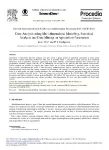
Multidimensional Visualization along the First Two Significant Dimensions
1 0.9 0.8 0.7 0.6 0.5 0.4 0.3 0.2 0.1 0
Given a pDView query, first, the relevant attributes of the data specified in the query are projected, clustered, and the counts for the unique combinations are computed. Let αi = ha1,i , . . . , ak,i i be an instance of R[A1 , . . . , Ak ]. αi is referred to as a context-instance. Let R(αi ) [Ak+1 , . . . , Am ] denote the portion of the table R containing the visualizationinstances corresponding to the context αi . Given a visualization-instance βj = hak+1,j , . . . , am,j i of the portion R(αi ) [Ak+1 , . . . , Am ], the value of count(i, j) is computed as | R(αi ) [Ak+1 = ak+1,j , . . . , Am = am,j ] |. A visualizationinstance frequency matrix VF, then, reports the frequency (normalized between 0 and 1) of each visualization-instance, βj = hak+1,j , . . . , am,j i, for each context instance, αi = ha1,i , . . . , ak,i i: VF(i, j) = count(i, j)/maxh {count(h, j)}. The second step in preparing the data for pDTree construction involves the identification of a basis consisting of a set of mutually independent unit vectors. This basis defines a space on which the relationships among visualizationinstances as well as context-instances can be studied. For this purpose, we use the well known Singular Value Decomposition approach (SVD [3]) on the VF matrix. SVD splits the input matrix into three matrices, VF = U ΣV t , such that U and V are column orthonormal matrices and Σ is a diagonal matrix. The advantage of SVD is that mutually independent columns of U and V can be considered as basis of the space on which visualization- and context-instances can be studied. Also, the weights of the diagonal entries of Σ can be considered as the significance of the corresponding
Dim2
2.1 Data Preparation
0
0.2
0.4
Dim1
0.6
0.8
1
Figure 2: A multidimensional visualization (along the most significant two dimensions) for the data set in Figure 1. Despite major dimensional losses, patterns (easily visible in the pDTree) are hard to discern.
columns in U and V .
2.2
Pattern Development Tree (pDTree)
SVD underlies many data analysis and dimensionality reduction techniques (such as latent semantic analysis [4]). On the other hand, while such principal component based study is highly common we note that it is not sufficient in itself for effective visualization of the data. In particular, the significance values computed by SVD enable reduction in the number of dimensions, but in many cases, the number of relevant dimensions is still beyond what can be visualized effectively. Furthermore, even if the data is compressed to very low-dimensional spaces (2D- or 3D-) to be displayed on screen, simply presenting the data points
1
0.45 C(3)
0.9
0.4 B(2)
0.8
(boundary #1)
A(1)
0.35
node1
0.7
0.3
E(5)
0.6
0.2
D(4)
0.4 0.3
0.15
0.2
0.1
0.1
0.05
0 0.6
A A A A A A A
(boundary #3) node8
0.25
0.5
0.65
→ B vs. →B→E → B → C vs.. →B→C→E → D vs.. →D→E vs. A → E
0.7
0.75
0.8
0.85
0.9
0.95
0 -0.05 0
1
node2
node9
Trend before segmentation
node7
node3
node10 (boundary #4)
0.1
node4
node6 (boundary #2)
0.2
0.3
0.4
node5
0.5
0.6
0.7
x-std diff.
y-std diff.
ang. diff
avg.
0.066
0.115
0.667
0.283
Figure 4: Partitioning of a non-uniform branch (from
0.011
0.068
0.808
0.296
0.066 0.191
0.082 0.141
0.833 0.638
0.327 0.323
node1 to node10) into segments: each partition acts as a coherent pattern in the data and only boundaries are considered for new branches
Figure 3: An example fpDTree of line segments: The new visualization instance, E, is connected to the a tree based on its compatibility to the existing branches. Here, E is most compatible with A → B
for scientist’s visual interpretation is not effective: in many cases, it is hard for the user to view the data from all relevant points-of-view to identify patterns implying strong relationships among the visualization-instances and/or the context-instances (Figure 2). Therefore, unlike most techniques which effectively amount to dimensionality reduction based on the available significance information, we go further and use the U , V , Σ matrices obtained through SVD to obtain a pattern development tree (pDTree), which does not suffer from the visualization shortcomings of the multidimensional spaces. Let us consider the matrix V which maps the visualization-instances onto a multidimensional space defined by the independent basis vectors. Let us call ~ on S, we this space, S. For each visualization-instance, vi, ~ compute a dominance value (dom(vi)), which describes how dominant the visualization-instance is in space S. We define ~ as follows: dom(vi) ~ = |vi ~ − h0, 0, . . . , 0i|. Intuthe dom(vi) itively, those visualization-instances that occur frequently (i.e., further away from the null point h0, 0, . . . , 0i) dominate the others. This interpretation is consistent with the observation that the extended boolean model of vector spaces [5] enables one to treat those vectors that are further away from the origin as being also more general [7]. This enables us to order the visualization-instances into a tree (where nodes higher up in the hierarchy are more general/dominant) based on their dominance values: the dominant visualization-instances (away from h0, 0, . . . , 0i) are mapped closer to the root. pDView can use two different strategies to create pDTrees: The free pattern development tree (fpDTree) strategy relies on the assertion that each branch of the tree represents a set of instances that collectively define a coherent (in terms of overall direction in the space and distribution of instances) pattern in the space. Therefore, new branches are created where instances violate existing patterns. The angular pattern development tree (apDTree) strategy, on the other hand, gives more emphasis on the relative value-compositions of
the instances and only places visualization-instances with similar compositions as part of the same branch.
2.2.1
Free Pattern Development Tree (fpDTree)
While dominance helps us order visualization-instances, it does not determine how branching is created in a pDTree. Intuitively, if two visualization-instances are related to each other within the current context of analysis, they need to be part of the same branch. In fpDTrees, each root-to-instance path is analyzed for pattern developments and shifts (including slope, concentration). For each visualization-instance, considered during the construction of the fpDTree, the most compatible branch of the current fpDTree is chosen as the connection point. Pattern development analysis underlying the branching decisions involves (a) analysis of the hypercurves (linear, planar, etc.) defined by branches of the trees, before and after the insertion of the new visualization instance, and (b) checking whether attaching the new visualization instance to that branch will cause a large deviation from the current characteristics of the branch. See Figure 3 for an example fpDTree of line segments. Note that, while this figure only illustrates fpDTree construction in terms of line segments, pDView analyzes planar and hyper-planar pattern developments simultaneously (without requiring exponential growth in analysis time). The user of pDView, then can pick the dimensionality of the pattern developments or have pDView to scale the number of dimensions needed to create the fpDTree as appropriate. For reducing the computational complexity of branching analysis during fpDTree construction as well as to prevent very long branches from causing deformations, fpDTree partitions long branches into coherent segments, using multidimensional hyper-curvature analysis [9, 8]. It considers only those identified segment boundaries as candidates for branching (Figure 4).
2.2.2
Angular Pattern Development Tree (apDTree)
Unlike the fpDTree which analyzes the pattern development along the various branches explicitly using multiple pattern development parameters, apDTree treats two visualizationinstances to be related only when they have similar compositions with respect to the basis of the underlying multidimensional space: while their dominance in the data set
Figure 5: Selection of context- and visualizationattributes.
Figure 7: The selection of a visualization-instance (Cottontail rabbit) triggers the ranking of the context-instances based on cosine similarity. tle Colorado prehistory project data set [1], consisting of a relation with ∼30,000 tuples on 20 attributes, and show how (a) the context of interest and the visualization attributes are interactively selected, as shown in Figure 5, (b) how the patterns on the visualization attributes are visualized in fPDTrees and aPDTrees as a function of the context (Figure 6 shows a fish-eye exploration view), and (c) how the user can focus on a node of the pDTree for further exploration tasks like manual or automatic selections of dimensions relevant to the pattern selected and visualized, or ranking of context-instances based on cosine similarity (Figure 7).
4.
ACKNOWLEDGMENTS
We thank Prof. Keith Kintigh for the data set and his help with the interpretations of the results.
5. Figure 6: Dynamic fish-eye view of the angular Pattern Development Tree created with the settings shown in Figure 5.
may differ significantly, such a pair of entries are related to the underlying context-instances in a similar manner. Thus, in apDTrees, for branch differentiation, we rely on the angular differences (i.e. difference in compositions) of the visualization-instances. Visualization-instances with similar compositions are part of the same branch of the apDTree, while visualization-instances with different compositions should be mapped onto different branches. To achieve this, we incrementally construct the apDTree by considering the visualization-instances in the decreasing order of their dominance values (as in fpDTrees) and by connect~ i , to the one, vi ~ j , most ing each visualization-instance, vi ~ i , vi ~ j )) similar (in terms of their compositions; i.e., cosine(vi already included in the apDTree. See Figure 1(a) for a sample angular pDTree created using a database containing different animal bone specimens collected at an archaeological site. Note that, except for a few mis-associations (which secondary linkage analysis -the dashed line- provided by pDView can reveal), the apDTree is almost a valid taxonomy of the species.
3. DEMO SCENARIO We demonstrate the pattern development view system for visualization of multidimensional data through its use in an archaeological domain. Specifically, we will use the Upper Lit-
REFERENCES
[1] T.C.Clark. Assessing Room Function Using Unmodified Faunal Bone: A Case Study from East-central Arizona. Kiva64(1): 1998. [2] G.Chintalapani, C. Plaisant, B.Shneiderman: Extending the Utility of Treemaps with Flexible Hierarchy. IV, 2004. [3] C. Eckart, G. Y. The Approximation of One Matrix by Another of Lower Rank. Psychometrika, 1936. [4] S. Deerwester, S. Dumais, G.Furnas, R. Harshman, T. Landauer, K. Lochbaum and L. Streeter. Computer Information Retrieval using latent semantic Structure, US Patent, 1989. [5] G. Salton, E.A. Fox, and H. Wu. Extended Boolean Information Retrieval. CACM, 26(11). 1983. [6] T. Jirka. Multidimensional Data Visualization, Technical Report (DCSE/TR-2003-03), 2003. [7] J.W. Kim and K.S. Candan. CP/CV: Concept Similarity Mining without Frequency Information from Domain Describing Taxonomies. CIKM, 2006. [8] David G. Lowe. Three-dimensional object recognition from single two-dimensional images. AI, 1987. [9] Y. Qi, K. S. Candan: CUTS: CUrvature-based Development Pattern Analysis and Segmentation for Blogs and other Text Streams. Hypertext, 2006. [10] J.Seo and B.Shn. A Rank-by-Feature Framework for Unsupervised Multidimensional Data Exploration Using Low Dimensional Projections. IV 2004.. [11] K. Techapichetvanich, A. Datta, Interactive Visualization for OLAP, LNCS, Vol. 3482, 2005.