Unsteady Vibration Aerodynamic Modeling and Evaluation of Dynamic ...

Hindawi Publishing Corporation Mathematical Problems in Engineering Volume 2015, Article ID 813462, 15 pages http://dx.doi.org/10.1155/2015/813462

Research Article Unsteady Vibration Aerodynamic Modeling and Evaluation of Dynamic Derivatives Using Computational Fluid Dynamics Xu Liu, Wei Liu, and Yunfei Zhao College of Aerospace Science and Engineering, National University of Defense Technology, Changsha 410073, China Correspondence should be addressed to Xu Liu; [email protected] Received 6 April 2015; Revised 10 July 2015; Accepted 26 July 2015 Academic Editor: Oded Gottlieb Copyright © 2015 Xu Liu et al. This is an open access article distributed under the Creative Commons Attribution License, which permits unrestricted use, distribution, and reproduction in any medium, provided the original work is properly cited. Unsteady aerodynamic system modeling is widely used to solve the dynamic stability problems encountering aircraft design. In this paper, single degree-of-freedom (SDF) vibration model and forced simple harmonic motion (SHM) model for dynamic derivative prediction are developed on the basis of modified Etkin model. In the light of the characteristics of SDF time domain solution, the free vibration identification methods for dynamic stability parameters are extended and applied to the time domain numerical simulation of blunted cone calibration model examples. The dynamic stability parameters by numerical identification are no more than 0.15% deviated from those by experimental simulation, confirming the correctness of SDF vibration model. The acceleration derivatives, rotary derivatives, and combination derivatives of Army-Navy Spinner Rocket are numerically identified by using unsteady N-S equation and solving different SHV patterns. Comparison with the experimental result of Army Ballistic Research Laboratories confirmed the correctness of the SHV model and dynamic derivative identification. The calculation result of forced SHM is better than that by the slender body theory of engineering approximation. SDF vibration model and SHM model for dynamic stability parameters provide a solution to the dynamic stability problem encountering aircraft design.

1. Introduction In aircraft design and development, it is difficult and costly to achieve dynamic stability within the flight envelop. Shock wave-induced separation, swirling motion and rupture, and the interaction between them lead to strong unsteady and nonlinear behaviors of fluid motion, which generally results in aerodynamic effect beyond expectation and even some overwhelming consequences [1]. In the aircraft design stage, it is hard to foresee the boundaries of dynamic operation stability and the severity level of dynamic problems, most of which are not discovered until in the flight test stage. This directly leads to multiplication of the aircraft design cycle, significant increase of design cost, and unavoidable aircraft performance loss in connection with local reshaping. Since the beginning of this century, dynamic stability problems have been a common phenomenon [2]. To better understand the causes of flight stability deterioration from the fluidity mechanism horizon, unsteady aerodynamic mathematic model has been widely applied to the studies on dynamic flight quality

issues [3]. A mature, reliable package of unsteady aerodynamic mathematic models enables us to evaluate and select different aircraft design plans so as to minimize the aircraft design cost and mitigate risk exposure [4]. In aircraft flight, atmospheric turbulence, asymmetric transition, base flow interference, maneuver implementation, and other disturbances can result in highly complex aerodynamic consequences such as asymmetric vortex separation, shedding or breakup, shock motion, and vortex or boundary layer disturbances, which eventually give rise to dynamic stability problems of the aircraft [5]. Longitudinal or lateral vibration amplitude and frequency vary linearly with the motion attitude angle and its variation rate: the vibration process can be either convergent or divergent. The vibration amplitude can span from a few to dozens of degrees or even be divergent [6]. These greatly affect the stability control and trajectory design of a hypersonic aircraft and even the imaging of the airborne camera. Severe dynamic behavior problems could cause the aircraft to disintegrate [2].

2

Mathematical Problems in Engineering

(a) Steady linear flight

(b) Static instability

(c) Static neutral stability

(d) Static stability, dynamic stability

(e) Static stability, dynamic neutral stability

(f) Static stability, dynamic instability

Figure 1: Five motion states of aircraft after disturbance.

In the hypersonic or supersonic stage, when a spacecraft reenters the atmosphere, it is often challenged by the rolling-helical modal coupling problem. In its X-33 research, the United States discovered that the lifting body it designed is noticeably laterally unstable in construction. All the validation projects implemented by the United States Defense Advanced Research Projects Agency (DARPA) and the United States Air Forces on Falcon hypersonic technology vehicle (HTV) ended up with failure [7], and all these failures are closely associated with the stability control of the aircraft attitude. The stability analysis result of University of Maryland suggests that the waverider aircraft tends to be longitudinally unstable under three hypersonic states [8]. The analysis report on the first flight failure of X-43A points out that the specially structured aerodynamic forces of the aircraft have far greater than expected nonlinearity, and the inaccurate aerodynamic modeling is considered to be one of the critical failure aspects [9]. Dynamic unsteady aerodynamic system modeling is widely used to solve these dynamic stability problems encountering aircraft design [4]. An unsteady aerodynamic

model is used to determine the motion state variables that decide aerodynamics and the relation among these variables. In this model, the aerodynamic load to which the aircraft is subject is expressed as the function of the motion state parameter and the transient value of its derivative [10]. The coefficients of the orders in the function are called dynamic derivatives, which directly decide the divergence feature of the aircraft open-loop system when oscillating under disturbance [11]. For a free flight aircraft, dynamic derivative prediction is indispensable and directly decides the flight stability. Figure 1 gives the five motion states of a free flight aircraft after disturbance. The stability of the aircraft closedloop system is not only decided by aerodynamic stability; it is also associated with the control system. The control system can change the system stability by feeding back the attitude plane and angular speed. Dynamic derivatives decide the gain factor of the control system. Excessive adjustment of the feedback gain can degrade the aircraft maneuverability and deteriorated controllability and flight qualities though good flight stability is guaranteed.

Mathematical Problems in Engineering

3

Table 1: Dynamic stability derivatives of the moment coefficient. Rotation derivatives Acceleration derivatives

Vibration around a fixed axis Damping derivatives Cross derivatives Cross-coupling derivatives

Roll moment derivatives

𝐶𝑙𝑝 , 𝐶𝑙𝑞 , 𝐶𝑙𝑟

𝐶𝑙𝛼̇ , 𝐶𝑙𝛽 ̇

𝐶𝑙𝑝 + 𝐶𝑙𝛽 ̇ sin 𝛼

Pitch moment derivatives

𝐶𝑚𝑝 , 𝐶𝑚𝑞 , 𝐶𝑚𝑟

𝐶𝑚𝛼̇ , 𝐶𝑚𝛽 ̇

𝐶𝑚𝑞 + 𝐶𝑚𝛼̇

Yaw moment derivatives

𝐶𝑛𝑝 , 𝐶𝑛𝑞 , 𝐶𝑛𝑟

𝐶𝑛𝛼̇ , 𝐶𝑛𝛽 ̇

𝐶𝑛𝑟 − 𝐶𝑛𝛽 ̇ cos 𝛼

The idea of stability and dynamic derivative was first proposed by Bryan [12] in 1911 and is still used today in some engineering problems as a conventional derivative model for aerodynamic load [10]. Over the hundred years’ history of unsteady aerodynamic mathematic model, one after another, modified models targeting at the shortfalls of Bryan model have been introduced. These include state space model [13] (differential equation model), indicating function model [14] (integral equation model), Etkin full-order model, and reduced-order model having gained rapid development over the past few years [15–17]. Table 1 lists the dynamic stability derivatives of the moment coefficient, where 𝐶𝑙 , 𝐶𝑚 , and 𝐶𝑛 represent rolling, pitching, and yawing moment coefficients, respectively; 𝛼 and 𝛽 are the angle of attack and angle of sideslip; 𝑝, 𝑞, and 𝑟 are the angular speed components of the rolling axis, pitching axis, and yawing axis. In our study, single degree-of-freedom (SDF) vibration model and forced simple harmonic motion (SHM) model for dynamic derivative prediction is developed on the basis of modified Etkin model [5]. To validate the predictions, two test cases are used. For blunted cone calibration model, the coupling computation between aircraft motion and flow field motion equations is studied using the unsteady SDF vibration model. For Army-Navy Spinner Rocket, dynamic derivatives at different positions of center of mass are identified by solving three-dimensional unsteady N-S equation and compared with the computational result of the United States Army Research Laboratory and experimental result of the United States Army Ballistic Research Laboratories.

𝐶𝑙𝑞 + 𝐶𝑙𝛼̇ 𝐶𝑚𝑟 − 𝐶𝑚𝛽 ̇ cos 𝛼 𝐶𝑚𝑝 + 𝐶𝑚𝛽 ̇ sin 𝛼

𝐶𝑛𝑝 + 𝐶𝑛𝛽 ̇ sin 𝛼

𝐶𝑛𝑞 + 𝐶𝑛𝛼̇

𝑈 = (𝑢, V, 𝑤)𝑇 . The total energy per unit mass is 𝑒. The inviscid flux vectors, 𝐸, 𝐹, and 𝐺, are given by 𝜌𝑢 𝜌𝑢2 + 𝑝

) ( 𝐸 = ( 𝜌𝑢V ) , 𝜌𝑢𝑤 ( 𝜌ℎ𝑢 ) 𝜌V 𝜌𝑢V ( 2 ) 𝐹 = (𝜌V + 𝑝) ,

(2)

𝜌V𝑤 ( 𝜌ℎV ) 𝜌𝑤 𝜌𝑢𝑤 ( 𝜌V𝑤 ) 𝐺=( ), 𝜌𝑤2 + 𝑝 ( 𝜌ℎ𝑤 ) while the viscous flux vectors, 𝐹V , 𝐺V , and 𝐻V , contain terms of the heat flux and viscous forces exerted on the body and can be represented by 𝐸V

2. Computational Fluid Dynamics Formulation Under the Cartesian inertial coordinate system, the threedimensional dimensionless Navier-Stokes equation for perfect gases with ignored mass forces is as follows: 𝜕𝑄 𝜕𝐸 𝜕𝐹 𝜕𝐺 𝜕𝐸V 𝜕𝐹V 𝜕𝐺V + + + = + + , 𝜕𝑡 𝜕𝑥 𝜕𝑦 𝜕𝑧 𝜕𝑥 𝜕𝑦 𝜕𝑧

𝐶𝑙𝑟 − 𝐶𝑙𝛽 ̇ cos 𝛼

(1)

where 𝑄 is the vector of conserved variables, 𝑄 = (𝜌, 𝜌𝑢, 𝜌V, 𝜌𝑤, 𝜌𝑒)𝑇 , 𝜌 is the density, and 𝑢, V, and 𝑤 are the components of velocity given by the Cartesian velocity vector

=

𝜕𝑇 𝑇 1 (0, 𝜏𝑥𝑥 , 𝜏𝑥𝑦 , 𝜏𝑥𝑧 , 𝑢𝜏𝑥𝑥 + V𝜏𝑥𝑦 + 𝑤𝜏𝑥𝑧 + 𝑘󸀠 ) Re 𝜕𝑥

𝐹V =

𝜕𝑇 𝑇 (3) 1 (0, 𝜏𝑦𝑥 , 𝜏𝑦𝑦 , 𝜏𝑦𝑧 , 𝑢𝜏𝑦𝑥 + V𝜏𝑦𝑦 + 𝑤𝜏𝑦𝑧 + 𝑘󸀠 ) Re 𝜕𝑦

𝐺V =

𝜕𝑇 𝑇 1 (0, 𝜏𝑧𝑥 , 𝜏𝑧𝑦 , 𝜏𝑧𝑧 , 𝑢𝜏𝑧𝑥 + V𝜏𝑧𝑦 + 𝑤𝜏𝑧𝑧 + 𝑘󸀠 ) . Re 𝜕𝑧

4

Mathematical Problems in Engineering

Here, 𝜏𝑖𝑗 is the stress tensor components. 𝑘󸀠 is the heat transfer coefficient. Consider 𝑘󸀠 =

𝜇 𝜇 1 ( 𝐿 + 𝑇 ). 2 Pr𝐿 Pr𝑇 (𝛾 − 1) 𝑀∞

(4)

Here, 𝛾 is the specific heat ratio. Pr𝐿 and Pr𝑇 are the laminar and turbulent Prandtl number. 𝑀∞ and Re are the freestream Mach number and Reynolds number, respectively. The Spalart-Allmaras (SA) model is employed to evaluate the turbulent viscosity 𝜇𝑇 . The laminar viscosity, 𝜇𝐿 , is evaluated using Sutherland’s law: 𝜇𝐿 = 𝑇3/2 (

1+𝑐 ), 𝑇+𝑐

(5)

110.4𝐾 . 𝑐= ̃∞ 𝑇

Second-order upwind NND scheme finite volume [18, 19] was used to discretize the spatial derivative term of the flow-controlled equation group. The LU-SGS containing dual time steps [20, 21] was used to obtain higher efficiency and precision of time solution. Rigid grid generation method where grids are fixedly connected to the object is used for unsteady dynamic calculation. When the object is in motion, the coordinate system remains unchanged while the grids, fixedly connected to the object, make rigid motion. The aircraft motion is decomposed into translation with the centroid and rotation with the centroid. Assume that the Euler angle sequence during aircraft rotation is pitching 𝜃, then yawing 𝜓, and then rolling 𝜙. The Euler angle direction is positive along the positive direction of the coordinate axis according to the right-hand rule. Record the centroid position at the initial time as (𝑥𝑜1 , 𝑦𝑜1 , 𝑧𝑜1 ), the aircraft centroid position at time 𝑡 as (𝑥𝑜2 , 𝑦𝑜2 , 𝑧𝑜2 ), and the Euler angle as (𝜃, 𝜓, 𝛾). Then, for any grid point at the initial time (𝑥0 , 𝑦0 , 𝑧0 ), the coordinate (𝑥1 , 𝑦1 , 𝑧1 ) at time 𝑡 is 𝑥1 − 𝑥𝑜2

𝑥0 − 𝑥𝑜1

(𝑦1 − 𝑦𝑜2 ) = 𝑀1 (𝜙) 𝑀2 (𝜓) 𝑀3 (𝜃) (𝑦0 − 𝑦𝑜1 ) , (6) 𝑧1 − 𝑧𝑜2

𝑧0 − 𝑧𝑜1

where 𝑀𝑖 is the elementary transformation matrix of the coordinate system. The greatest merit of dynamic grids generated by this method is that they are simple and applicable for unsteady motions of any configuration and any amplitude. Dynamic grids are as good as static grids and conform to geometric conservation law. For dynamic unsteady calculation, far-field boundaries were treated with nonreflecting boundary conditions (NRBC) based on Riemann variable and applicable for dynamic movement. For wall boundary, the velocity was accounted for nonslip conditions, the temperature was accounted for diathermic wall, and the pressure conditions accounted for centrifugal forces.

3. Single Degree-of-Freedom Vibration Modeling The free pitch motion of aircraft around the fixed axis is expressed by the equation for rigid body rotation with a fixed axis: 𝐼𝑧𝑧 𝜃̈ = 𝐶𝑚 + 𝜇𝑧 𝜃.̇

(7)

Here, 𝐼𝑧𝑧 is the dimensionless moment of inertia; 𝜇𝑧 is the dimensionless mechanical damping coefficient; 𝜃 is the angle of pitch starting from the balance point. When flight aerodynamics discusses the dynamic stability of aircraft under disturbance, the aerodynamic forces on the aircraft are expressed as the linear function of the motion dynamic parameters [22]. For SDF pitch motion, under the hypothesis of Etkin’s aerodynamic model [5], the pitch moment coefficient 𝐶𝑚 can be expressed as 𝐶𝑚 (𝑡) = 𝐶𝑚 [𝛼 (𝑡) , 𝛼̇ (𝑡) , 𝛼̈ (𝑡) , . . . , 𝑞 (𝑡) , 𝑞 ̇ (𝑡) , 𝑞 ̈ (𝑡) , . . .] .

(8)

Here, 𝛼, 𝛼,̇ 𝛼,̈ . . . are the derivatives of orders of the angle of attack and its time; 𝑞, 𝑞,̇ 𝑞,̈ . . . are the derivatives of orders of the pitch angular speed and its time. For (8), Taylor series expansion is performed at the balance angle of attack (omitting the high-order terms): 𝐶𝑚 = (𝐶𝑚𝛼 )0 𝜃 + (𝐶𝑚𝑞 + 𝐶𝑚 𝛼̇ )0 𝜃.̇

(9)

Here, (𝐶𝑚𝛼 )0 and (𝐶𝑚𝑞 + 𝐶𝑚 𝛼̇ )0 are the pitch rigidity and pitch damping derivatives at the balance angle of attack. From (9), the free vibration of aircraft is not only subject to aerodynamic recovery moment due to deviation from the balance angle of attack, but also subject to the air damping moment caused by changes in the angle of attack or the angle of pitch [10]. Substitute (9) into (7) and we get the secondorder differential equation for aircraft SDF vibration: 𝐼𝑧𝑧 𝜃̈ − [(𝐶𝑚𝑞 + 𝐶𝑚 𝛼̇ )0 + 𝜇𝑧 ] 𝜃̇ − (𝐶𝑚𝛼 )0 𝜃 = 0.

(10)

When giving the analytic solution to this differential equation, we regard (𝐶𝑚𝑞 + 𝐶𝑚𝛼̇ )0 as a constant and (10) as a constant coefficient linear differential equation. 3.1. Small Damping Modal. For the small damping modal, the roots of its characteristic equation are a conjugate complex root pair. Hence the general solution to (10) is 𝜃 = 𝐴𝑒𝜆𝑡 cos (𝜔𝑡 + 𝜑) .

(11)

From (11), the motion of an object is a vibration over the time cycle 𝑇 = 2𝜋/𝜔. However, different from simple harmonic vibration (SHV), its amplitude 𝐴𝑒𝜆𝑡 varies

Mathematical Problems in Engineering

5

𝜃

𝜃

t

t

(a) Amplitude attenuated

(b) Amplitude unchanged

𝜃

t

(c) Amplitude diverged

Figure 2: Vibration at small damping modal.

exponentially with time 𝑡 as shown in Figure 2. The envelop line equation connected by angular amplitudes is 𝜃 = 𝜃0 𝑒𝜆𝑡 = 𝜃0 𝑒[(𝐶𝑚 𝑞 +𝐶𝑚 𝛼̇ )0 +𝜇𝑧 ]𝑡/2𝐼𝑧𝑧 .

(12)

As in numerical calculation, 𝜇𝑧 = 0, when (i) (𝐶𝑚𝑞 +𝐶𝑚 𝛼̇ )0 < 0, the amplitude attenuates representing dynamic stability as shown in Figure 2(a); (ii) (𝐶𝑚𝑞 + 𝐶𝑚 𝛼̇ )0 = 0, the amplitude stays unchanged representing dynamic neutral stability as shown in Figure 2(b); (iii) (𝐶𝑚𝑞 + 𝐶𝑚 𝛼̇ )0 > 0, the amplitude increases representing dynamic instability as shown in Figure 2(c). By numerically simulating the free pitch process of aircraft, we get the time-related function curve of angle of pitch as shown in Figure 3. The function expression of this curve has been obtained from the analysis above (11).

𝜃0,1 𝜃0,2

𝜃

T

2T t

Figure 3: Dynamic derivative identification curve of pitch angular vibration.

6

Mathematical Problems in Engineering

𝜃

𝜃

0

t (a) Amplitude attenuated

0

t (b) Amplitude diverged

Figure 4: Vibration at large damping modal.

Select angles of pitch from the curve one time cycle apart from each other, 𝜃1 and 𝜃2 (corresponding to 𝑡1 and 𝑡2 , and 𝑡2 = 𝑡1 + 𝑇): 𝜃1 = 𝐴𝑒𝜆𝑡1 cos (𝜔𝑡1 + 𝜑) , 𝜆𝑡2

𝜃2 = 𝐴𝑒

𝜆𝑡2

cos (𝜔𝑡2 + 𝜑) = 𝐴𝑒

cos (𝜔𝑡1 + 𝜑 + 2𝜋) .

(13)

By dividing them, we get 2𝐼 𝜃 (𝐶𝑚𝑞 + 𝐶𝑚 𝛼̇ )0 = 𝑧𝑧 ln 2 − 𝜇𝑧 . 𝑇 𝜃1

Δ𝛼1 Δ𝛼̇1 Δ𝛼2 Δ𝛼̇2 A=( . .. ) . .. .

(14)

(15)

Here, arbitrary constants 𝑐1 and 𝑐2 can be determined by the initial conditions. If static stability is included, we have 𝑟1,2 < 0. From (15), there is a maximum of one 𝑡 that makes 𝜃 = 0. That is, the object can cross over the balance point one time at most. Hence the object does not vibrate anymore. The function graph is as shown in Figure 4. Dynamic stability parameters are solved using a linear regression model. Define independent variable x and dependent variable y:

Using linear regression process for solution, we get (A𝑇A) x = A𝑇 y.

y=(

3.3. Critical Damping Modal. For the critical damping modal, its characteristic equation has two unequal real roots: 𝑟1,2 =

𝐶𝑚 (𝑡2 ) − 𝐶𝑚0 .. .

(18)

Normally, matrix A is not a square array and has more rows than columns. Many numerical methods can solve this least square (LS) problem [23]. These include direct transposition A𝑇A, Gaussian elimination method, MoorePenrose generalized inversion method, and QR factorization though Moore-Penrose generalized inversion method and QR factorization are more accurate than direct transposition and Gaussian elimination. In terms of calculation quantity, it is 𝑂(𝑛2 ) for QR factorization and 𝑂(𝑛3 ) for Moore-Penrose generalized inversion method.

𝐶𝑚𝜃 ), x=( 𝐶𝑚𝜃̇ 𝐶𝑚 (𝑡1 ) − 𝐶𝑚0

(17)

Δ𝛼𝑁 Δ𝛼̇𝑁

3.2. Large Damping Modal. For the large damping modal, its characteristic equation has two unequal real roots. The general solution to the equation is 𝜃 = 𝑐1 𝑒𝑟1 𝑡 + 𝑐2 𝑒𝑟2 𝑡 .

Matrix A that associates the unknown parameters and dependent variable is defined as

𝑀𝛼̇ . 2𝐼𝑧𝑧

(19)

The general solution to the equation is (16) ).

(𝐶𝑚 (𝑡𝑁) − 𝐶𝑚0 )

𝜃 = 𝑒𝜆𝑡 (𝑐1 + 𝑐2 𝑡) , 𝜆=

(𝐶𝑚𝑞 + 𝐶𝑚 𝛼̇ )0 + 𝜇𝑧 2𝐼𝑧𝑧

(20) .

Mathematical Problems in Engineering

7

Figure 5: Forced pitching vibration of aircraft.

Figure 6: Forced plunging vibration of aircraft.

Figure 7: Forced flapping vibration of aircraft.

Arbitrary constants 𝑐1 and 𝑐2 can be determined by the initial conditions. From (20), there is a maximum of one 𝑡 that makes 𝜃 = 0. Hence the object does not vibrate any more.

4. Forced Simple Harmonic Motion Modeling Figures 5–7 show the aircraft flight attitudes and motion profiles under three types forced SHV (pitching/plunging/flapping). Forced pitching SHV is used to calculate the pitch direct damping derivative 𝐶𝑚𝑞 + 𝐶𝑚𝛼̇ , the vibration equation of which is 𝛼 (𝑡) = 𝛼0 + 𝜃 (𝑡) , 𝜃 (𝑡) = 𝜃𝑚 sin (𝑘𝑡) .

𝜃 (𝑡) = 0.

𝜃 (𝑡) = 𝜃𝑚 sin (𝑘𝑡) .

(24)

Here

(22)

Forced flapping SHV is used to calculate the rotary derivative of pitch moment 𝐶𝑚𝑞 , the vibration equation of which is 𝛼 (𝑡) = 𝛼0 ,

𝐶𝑚 (𝑡) = 𝐶𝑚0 + 𝐶𝑚𝜃 Δ𝜃 + 𝐶𝑚𝜃̇Δ𝜃.̇

(21)

Here, 𝛼0 is the initial angle of attack; 𝜃𝑚 is the pitch angle amplitude; 𝑘 is the dimensionless reduced frequency (𝑘 = ̃ is the circular frequency; 𝐿 ref is the ̃ ref /(2𝑉∞ ), where 𝜔 𝜔𝐿 reference length; 𝑉∞ is the inflow velocity). Forced plunging SHV is used to calculate the acceleration derivative of pitch moment 𝐶𝑚𝛼̇ , the vibration equation of which is 𝛼 (𝑡) = 𝛼0 + 𝛼𝑚 sin (𝑘𝑡) ,

the pitch direct damping coefficient 𝐶𝑚𝑞 + 𝐶𝑚𝛼̇ is calculated using pitching SHV. For aircraft under SHM, when the dynamic flow field reaches the periodical solution, it means the disturbance started infinitely long time ago, and modified Etkin model [5] does not include time 𝑡 as the explicit state-dependent variable. In such case, the state variables of the rolling round pitch axis motion are 𝛼 and 𝑞. As the base flight state is symmetric straight linear flight and subject to very modest disturbance amplitude, only first-order dynamic derivatives are included in the calculation. By performing Taylor expansion on (8) and ignoring small quantities of higher orders, we have

(23)

The superposition of plunging vibration and flapping vibration equals pitching SHV. In the next paragraphs,

𝐶𝑚𝜃 = 𝐶𝑚𝛼 − 𝑘2 (𝐶𝑚𝛼̈ + 𝐶𝑚𝑞̇) + 𝑘4 (𝐶𝑚𝛼... + 𝐶𝑚𝑞... ) −⋅⋅⋅ ,

(25)

𝐶𝑚𝜃̇ = (𝐶𝑚𝛼̇ + 𝐶𝑚𝑞 ) − 𝑘2 (𝐶𝑚𝛼... + 𝐶𝑚𝑞̈) + ⋅ ⋅ ⋅ . 𝐶𝑚𝜃 and 𝐶𝑚𝜃̇ are the in-phase and out-phase components of Δ𝐶𝑚 [24]. The resulting time domain data are postprocessed using formula (25) to identify the dynamic derivatives. Methods to realize this include integral method, domain frequency transformation, and phase method. In our example, the postprocessing results by integral method, frequency domain transformation, and phase method do not show significant divergence. Under a small reduced frequency, however, domain frequency transformation provides more accurate result than other methods. Phase method, which uses only two points of the time domain data, provides lower calculation accuracy and is thereby less frequently used.

8

Mathematical Problems in Engineering

4.1. Integral Method. Integral method derives 𝐶𝑚𝜃 and 𝐶𝑚𝜃̇ by calculating the first Fourier coefficient of Δ𝐶𝑚 over the time history of the first cycle 𝑇: 𝐶𝑚𝜃 = 𝐶𝑚𝜃̇ =

𝑡𝑠 +𝑇 𝑘 𝐶𝑚 (𝑡) sin 𝑘𝑡 𝑑𝑡 ∫ 𝜋𝛼𝑚 𝑡𝑠 𝑡𝑠 +𝑇

1 ∫ 𝜋𝛼𝑚 𝑡𝑠

(26)

𝐶𝑚 (𝑡) cos 𝑘𝑡 𝑑𝑡.

From (25) we can see that the frequency effect of the inphase component 𝐶𝑚𝜃 is significantly greater than the outphase component 𝐶𝑚𝜃̇. As the order of magnitude of the high-order coefficient 𝐶𝑚𝛼̈ + 𝐶𝑚𝑞̇, 𝐶𝑚𝛼... + 𝐶𝑚𝑞̈, 𝐶𝑚𝛼... + 𝐶𝑚𝑞... , . . . quickly reduces with the increase of the order of derivative. By ignoring the influence of the high-order coefficient and frequency effect, we can approximate to 𝐶𝑚𝜃 ≈ 𝐶𝑚𝛼 , 𝐶𝑚𝜃̇ ≈ 𝐶𝑚𝛼̇ + 𝐶𝑚𝑞 .

(27)

The in-phase/out-phase component approximation (27) applies to the extent that the aircraft flies at a small angle of attack under linear aerodynamic conditions, when the inphase and out-phase components are able to approximate the static derivative and combination derivative. When the flight is at a large angle of attack or subject to significant frequency effect, the influence of the highorder term coefficient is not ignorable [24, 25]. However, it is noted that when high-order coefficient is needed to express aerodynamics, as the orthogonal nature of model sequence itself keeps the fundamental harmonic unchanged, in-phase and out-phase components are still very important terms in aerodynamic expressions. When the flight is in an area subject to high nonlinear, unsteady aerodynamics, there can be a problem with the applicability of linearized model. In such case, a more advanced mathematic model [26–28] is needed to express the nonlinear, unsteady aerodynamics. 4.2. Frequency Domain Transformation. Frequency domain analysis has many merits and is applied to different areas. By transforming the frequency domain that acts on one cycle of stable harmonic, it is possible to obtain the frequency spectral characteristics of the aerodynamics and its in-phase/outphase components [29]. The finite Fourier integer of a continuous time scalar function 𝑥(𝑡) within a definite time interval 𝑡 ∈ [0, 𝑡] is defined as 𝑇

F [𝑥 (𝑡)] ≡ 𝑥 (𝑖𝜔) = ∫ 𝑥 (𝑡) 𝑒−𝑖2𝜋𝑓𝑡 𝑑𝑡. 0

(28)

Here 𝑖 is an imaginary unit and 𝑓 is the spatial frequency. Finite Fourier integer can be calculated at the discrete frequency 𝑓𝑘 , which is equal spaced from zero frequency through to Nyquist frequency 𝑓𝑁. Its frequency resolution is the reciprocal of the time step length [30]. The solution of any frequency on a given wave band can be obtained by linear frequency modulation 𝑍 transformation [31]. The amplitude

ratio and phase angle closely related to input signals in the system response can be determined by the transfer function of input and output. For pitch moment coefficient, the transfer function of pitch moment coefficient is [1] 𝐺 (𝑖𝜔) =

F [𝐶𝑚 (𝑡)] = 𝑅 (𝜔) 𝑒𝑖𝜙(𝜔) . F [𝛼 (𝑡)]

(29)

4.3. Phase Method. When forcing the aircraft to make smallamplitude, low-frequency SHV, perform Fourier expansion on the unsteady pitch moment 𝐶𝑚 : 𝐶𝑚 (𝑡) = 𝐶𝑚0 + 𝐶𝑚 sin (𝑘𝑡 + 𝜏) + 𝑢 (𝑡) .

(30)

Here 𝐶𝑚 is the aerodynamic force/moment amplitude of the fundamental harmonic component; 𝜏 is the phase angle between the displacement and aerodynamic moment of the aircraft when under forced vibration; 𝑢(𝑡) is the high-order harmonic component. To the extent that the unsteady calculation time is long enough and the calculation cycle 𝑛 is large enough, the influence of the initial effect is ignorable and the aerodynamic force/moment reaches a periodical steady-state value. Ordering 𝑘𝑡 = 2𝑛𝜋 + 0.5𝜋 (𝑛 = 1, 2, 3, . . .), we have 𝐶𝑚𝜃 =

𝐶𝑚 sin (𝜏 + (1/2) 𝜋) 𝜃𝑚

𝐶 [(4𝑛 + 1) 𝜋/2𝑘] − 𝐶𝑚0 = 𝑚 . 𝜃𝑚

(31)

Ordering 𝑘𝑡 = 2𝑛𝜋 (𝑛 = 1, 2, 3, . . .), we have 𝐶 𝑚𝜃 ̇ =

𝐶𝑚 sin 𝜏 𝐶𝑚 (2𝑛𝜋/𝑘) − 𝐶𝑚0 = . 𝑘𝜃𝑚 𝑘𝜃𝑚

(32)

5. Pitching Motion Stability of Blunted Cone 5.1. Computational Model and Conditions. For the 10-degree blunted cone calibration model, the bottom diameter is 𝑑 = 133.35 mm and bluntness ratio is 𝑟𝑛 /𝑟𝑏 = 0.4. Inflow conditions are as follows: 𝑀∞ = 4.0, Reynolds number based on bottom diameter Re𝑑 = 1.0 × 106 , 𝛼0 = 4∘ , 8∘ , 12∘ , and ̃∞ = 56.7 K. 𝑇 Three groups of examples are included. The first group uses different angular amplitudes (𝛼0 = 4∘ , 𝛼0 = 8∘ , and 𝛼0 = 12∘ ) to examine the effect of initial angular amplitude. The second group uses different centroid positions (𝑋𝑐𝑔 = 0.6040, 𝑋𝑐𝑔 = 0.6336, and 𝑋𝑐𝑔 = 0.6618) to examine the effect of vibration axis position. The third uses different moments of inertia (𝐼𝑧𝑧 = 0.01, 𝐼𝑧𝑧 = 0.1, and 𝐼𝑧𝑧 = 1) to examine the effect of moment of inertia and also compares the results between free vibration and forced vibration. 5.2. Computational Grids. The calculation mesh is shown in Figure 8. The number of cells is 99 × 73 × 57 (flow direction × circumferential × normal). The minimum cell distance is 0.92 × 10−4 𝑅𝑛 (𝑅𝑛 is the head radius). To examine the effect of grid density on the calculation result, the grids are refined

Mathematical Problems in Engineering

9

(a) 3D mesh

(b) Rear view of mesh

Figure 8: Mesh of a 10-degree blunted cone calibration model.

13

0.09

6

0.01

6

0.01

𝛼 −1

−8

0

5

10

15

Cmm

0.09

Cmm

13

𝛼

−0.07

−1

−0.15

−8 −25

−0.07

−15

t 𝛼 Cmm Fine mesh

−5 d𝜃/dt

5

−0.15 15

𝛼 Cmm Fine mesh

Figure 9: Free vibration time history of a blunted cone calibration model.

Figure 10: Free vibration phase curve of a blunted cone calibration model.

onefold in all the three directions into fine grids. The number of flow direction × circumferential × normal grids is 197 × 145 × 113. The total number of grids is eight times that of the previous grids. The free pitch process of the cone is numerically simulated. By solving the SDF vibration model, the time history and phase curve of the free vibration of the blunted cone calibration model are derived as shown in Figures 9 and 10. From these charts we can see that the blunted cone calibration model belongs to a small damping modal. It takes 22 hours to calculate one state of coarse grids using single process

method. The calculation result from fine grids in the chart is completely the same as that from coarse grids, suggesting that the density of coarse grids is enough for calculating unsteady aerodynamic and aerodynamic damping derivatives. 5.3. Flow Field Characteristics of Blunt Cone Configuration. Figures 11 and 12 give the pressure distribution and surface limiting streamline at the angle of attack of 12 degrees. The shock waves on the windward side moved toward the wall while those on the leeside elevated as a result of the angle of attack and the exposure of their strength to expansion waves

10

Mathematical Problems in Engineering Y

−1

0.8653 0.7136 X

Z

−0.9

0.5885 0.4853 0.4002 0.2722 0.2245 p 0.1851

(Cmq + Cm𝛼̇ )0

−0.8

0.3301

−0.7

+

+

+

−0.6

0.1527 0.1259

−0.5

0.1038 0.0856

−0.4

0.0706

2

6

10 𝛼0 (deg.)

0.0582

Figure 11: Pressure distribution cloud of symmetric plane.

Y

0.8655

+

14

18

CFD (free oscillation) Exp. (Prislin)

Figure 13: Effect of initial angular amplitude on obtaining pitching damping derivative by free vibration approach.

0.7142 X Z

0.5894 0.4864

−0.8

0.4013 0.3312

−0.75

0.2733 0.2255 p

0.1267 0.1046 0.0863 0.0712

(Cmq + Cm𝛼̇ )0

0.1536

+

−0.7

0.1861

−0.65 + −0.6

0.0588

Figure 12: Pressure spatial distribution and surface limiting streamline.

+

−0.55

−0.5 0.58

gradually decreased. After the shock, the direction and speed of the flow field changed. From the pressure cloud at the angle of attack of 12 degrees, we can clearly see the distribution of bow shocks and Mach waves. 5.4. Dynamic Stability of Blunt Cone Configuration. Figure 13 shows the effect of initial angular amplitude 𝛼0 on pitching damping derivative. Here, “+,” which is the computational point of our thesis, is obtained assuming 𝐼𝑧𝑧 = 0.1 and 𝑋𝑐𝑔 = 0.6040. Experiment [32] indicates that, for large bluntness ratio, 10-degree cone configuration (e.g., 𝑟𝑛 /𝑟𝑏 = 0.4), the difference of initial angular amplitude does not make much difference to dynamic stability. As can be observed from the chart, the calculation result agrees well with the experiment. The variation of (𝐶𝑚𝛼̇ + 𝐶𝑚𝑞 )0 with initial angular amplitude is insignificant.

0.62

0.66

0.7

Xcg = (0.6040, 0.6336, 0.6618)l

+

CFD (free oscillation) Exp. (Prislin)

Figure 14: Effect of vibration axis position on obtaining pitching damping derivative by free vibration approach.

In Figure 14, the lateral axis is the axis position of free vibration, taken as 𝑋𝑐𝑔 = 0.6040𝑙, 𝑋𝑐𝑔 = 0.6336𝑙, and 𝑋𝑐𝑔 = 0.6618𝑙, respectively. The longitudinal axis is the pitching damping derivative. “+” is the result of our calculation, assuming 𝐼𝑧𝑧 = 0.1, 𝛼0 = 12∘ . We can see that as the axis moves backward, the dynamic stability reduces. Our numerical calculation agrees well with the experiment.

Mathematical Problems in Engineering

11 14

15

12 10 8

9

6 𝛼

𝛼

4 2

3

0 −2 −3 −0.5

0

0.5

1

1.5

−4

2

0

0.5

1 t

t (a) 𝐼𝑧𝑧 = 0.001

1.5

2

(b) 𝐼𝑧𝑧 = 0.01

15

15

10

10

5 5 𝛼

𝛼

0

0 −5 −5

−10

−10

0

5

−15

10

0

10

20

30

40

50

60

70

t

t (c) 𝐼𝑧𝑧 = 0.1

(d) 𝐼𝑧𝑧 = 1

Figure 15: Free vibration configuration under increased moment of inertia.

Assuming the maximum angular amplitude 𝛼0 = 12∘ and 𝑋𝑐𝑔 = 0.6040𝑙, the free pitching process of the 10-degree blunt cone is numerically simulated at 𝐼𝑧𝑧 = 0.1, 0.01, 0.1 and 1. The corresponding angles of pitch variations are shown in Figures 15(a)∼15(d). From the profile of the curves, as 𝐼𝑧𝑧 increases, the amplitude attenuation becomes slower and slower, and the vibration period extends gradually. At this time, 𝜆 and 𝜔 in (11) are 𝜆=

(𝐶𝑚𝑞 + 𝐶𝑚 𝛼̇ )0 + 𝜇𝑧 2𝐼𝑧𝑧

󵄨󵄨 󵄨󵄨 2 󵄨󵄨 (𝐶 + 𝐶 ) + 𝜇 󵄨󵄨 ) (𝐶 𝑚𝑞 𝑚 𝑧 ̇ 𝛼 󵄨 𝑚𝛼 0 0 󵄨󵄨󵄨 ] + 𝜔 = √ 󵄨󵄨󵄨󵄨[ 󵄨. 2𝐼𝑧𝑧 𝐼𝑧𝑧 󵄨󵄨󵄨 󵄨󵄨 󵄨󵄨[ 󵄨󵄨 ]

(33)

We can see that when 𝐼𝑧𝑧 increases, the absolute of 𝜆 reduces and causes the amplitude to attenuate more slowly. The reduction of 𝜔 also leads to a longer vibration period. When 𝐼𝑧𝑧 is too small, overdamping occurs in Figure 15(a), preventing the curve from vibrating. After investigating the effect of moment of inertia, we compared free vibration with forced vibration. The amplitude of forced vibration is 1∘ . The vibration frequency is provided by free vibration. Vibration frequencies are read out from Figures 15(b)–15(d); that is, 𝐼𝑧𝑧 = 0.01, 𝐼𝑧𝑧 = 0.1, and 𝐼𝑧𝑧 = 1 correspond with frequencies 𝑘 = 6.91, 𝑘 = 2.33, and 𝑘 = 0.75. The calculation results are listed in Table 2. The two methods agree well with each other in terms of pitching rigidity, but the pitching damping derivatives vary a little bit significantly. However, as the vibration frequency reduces, the two calculations are closer to each other.

12

Mathematical Problems in Engineering

Table 2: Comparison of calculation results between free vibration and forced vibration. 𝑀∞ = 4, Re𝑑 = 1.0 × 106 , 𝛼0 = 12∘ , 𝑋𝑐𝑔 = 0.6040 Free/forced vibration −(𝐶𝑚𝑞 + 𝐶𝑚 𝛼̇ )0 −(𝐶𝑚𝛼 )0 Frequency 1 Frequency 2 Frequency 3

𝐼𝑧𝑧 = 0.01 𝑘 = 6.91 𝐼𝑧𝑧 = 0.1 𝑘 = 2.33 𝐼𝑧𝑧 = 1 𝑘 = 0.75

0.651 0.581 0.696 0.621 0.707 0.641

0.665 0.617 0.563 0.569 0.556 0.556

Table 3: Position of ANSR center of mass. Length of ANSR 5 9

Position of center of mass 3.0 3.5 5.038 5.885

2.5 4.0

7.0 3.0

2.0

1.0

8.5R 3.046

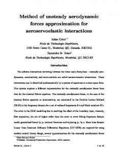
6. CFD Predictions of Dynamic Derivatives for Army-Navy Spinner Rocket 6.1. Computational Model and Conditions. The validation example is the Army-Navy Spinner Rocket (ANSR). A number of dynamic stability derivative experiments and calculations have been carried out targeting at the shape of ANSR calibration models [33–36]. Figure 16 shows the dimensions of the 5-caliber and 9-caliber ANSR calibration models, where the length of one caliber is 20 mm. In our study, the acceleration derivative, rotary derivative, and combination derivative of 5-caliber and 9-caliber ANSR calibration models along the pitch direction at the Mach number of 2.5 are identified. The correctness of the algorithm is validated by comparing calculations and experiments. Besides, the influence of the position of center of mass on the damping derivative is investigated by selecting three different positions of center of mass (see Table 3) for the calibration models. Here, one caliber equals 20 mm. For all the examples, the initial angles of attack and angles of sideslip are zero degrees. The free flow conditions are taken as the sea level conditions under standard atmosphere (101.325 kPa, 288 K). 6.2. Computational Grids. The three-dimensional calculation mesh is generated by rotating the symmetric plane mesh. Figure 17 shows the symmetric plane mesh near the rocket and topological structure. The numbers of cells of the 5caliber and 9-caliber ANSR calibration meshes are 275,000 and 296,000. The scale of the first layer of normal mesh is 10−5 𝐷, where 𝐷 is the rocket diameter. A small cell Reynolds number of around 10 is maintained. The mesh extension ratio near the head is limited to 1.1 maximum. To examine the effect of grid density on the calculation result, the grids are refined threefold in all the three directions into fine grids. The total number of grids is eight times that of the previous grids. Figure 18 shows the time history and hysteresis loop curves of pitching moment coefficient of 5-caliber ANSR model when its centroid position is 3.5. When the initial transient disturbance of forced pitching SHM deteriorates, the flow parameters and aerodynamic load come to harmonic, as shown in Figure 18(a). In Figure 18(b), the hysteresis loop under dynamic conditions appears to be smoothly inclined ellipse. The hysteresis loop area indicates the level of contribution of environment during the vibration

Figure 16: ANSR dimensions.

Figure 17: ANSR symmetric plane mesh topology.

of the projectile. The rotation direction of the hysteresis loop of plunging motion is also marked. The rotation direction of a hysteresis loop represents the direction of such work. Anticlockwise rotation means the work of the projectile on the environment, which consumes the dynamic energy of the projectile and contributes to dynamic stability. It takes 3 hours to calculate one state of coarse grids using 4-process parallel method. In the chart, the calculation result from fine grids fully agrees with that from coarse grids, suggesting that the density of coarse grids is enough for calculating unsteady aerodynamic and aerodynamic damping derivatives. 6.3. Dynamic Derivative Simulation Result of ANSR. Figure 19 compares the calculation result of our study (CFD), the referenced [36] result (PNS, SBT), and the referenced [34] experimental result (EXP) for the longitudinal derivatives of the ANSR calibration models. In our study, forced vibration is used to obtain the acceleration derivative 𝐶𝑚𝑎̇ , 𝐶𝑁𝑎̇ and combination derivative 𝐶𝑚𝑎̇ +𝐶𝑚𝑞 , 𝐶𝑁𝑎̇ +𝐶𝑁𝑞 . The forced vibration amplitude is one degree and the dimensionless reduced frequency 𝑘 is taken as 0.1. Quasi-steady method is used to obtain the rotary derivative 𝐶𝑚𝑞 , 𝐶𝑁𝑞 . By directly adding 𝐶𝑚𝑞 and acceleration derivative 𝐶𝑚𝑎̇ , we get 𝐶𝑚𝑎̇ + 𝐶𝑚𝑞 . Table 4 compares it with the combination derivative by forced vibration method, where the difference is not more than 2%, suggesting that the aerodynamics under these conditions satisfy the assumption of linear superposition. The main aerodynamic parametric variations are linear to the disturbance quantity.

13

0.1

0.1

0.05

0.05

Cmm

Cmm

Mathematical Problems in Engineering

0

−0.05

−0.1

0

−0.05

0

52

104

156

−0.1 −1.2

0.4

−0.4

t

1.2

𝛼

Cmm Fine mesh

Cmm Fine mesh (a) Time history curve

(b) Hysteresis loop

Figure 18: Time history curve and hysteresis loop of the pitching moment coefficient.

Table 4: Comparison of ANSR combination derivatives. c.g. 2.5 3.0 3.5 4.0 5.038 5.885

𝐶𝑚𝑎̇ + 𝐶𝑚𝑞 −25.71 −23.78 −24.62 −138.54 −118.94 −114.80

𝐶𝑚𝑎̇ + 𝐶𝑚𝑞 −25.85 −23.79 −25.02 −138.22 −119.39 −114.92

diff. 0.54% 0.04% 1.62% 0.23% 0.38% 0.10%

In Figure 19, PNS is the longitudinal dynamic stability derivative obtained by a British name Qin and Paul Weinacht from Army Research Laboratory when solving coning motion and helical motion in a noninertia system using parabolic N-S equation [36]. The merit of this method lies in its high efficiency that directly obtains the component forms of the combination derivative (acceleration derivative and rotary derivative). Its shortfall, however, lies in that it only applies to the small angle-of-attack linear state of an axial symmetric or planar symmetric shape and can only calculate the pitching and yawing channels. SBT is the result by the slender body theory of engineering approximation [36]. Except where the position of center of mass is 2.5-caliber at which time the pitch moment derivatives are the same as the CFD calculations, there are order of magnitude and even symbol differences in all the other states. EXP is the experimental result of the pitch moment combination derivative by the United States Army Ballistic Research Laboratories [34]. Engineering method SBT conforms to the experiment in terms of the dynamic derivative prediction trend, but the

numerical difference is significant. PNS method has the same results as our CFD calculation and experiment, validating the correctness of our method. For the pitch moment derivative of ANSR models, the proportion of the acceleration derivative representing flowing time lag effect is highly variable and can be as high as 40%–50%. However, as the center of mass shifts backwards, this proportion gradually reduces and is even opposite to the combination derivative symbol, contributing to dynamic instability. For the normal force derivative of ANSR models, the rotary derivative is linear to the position of center of mass while the acceleration derivative is not subject to the position of center of mass. The proportion of the acceleration derivative in the combination derivative is larger than that of the rotary derivative.

7. Conclusions A forced SHM model and SDF vibration model are developed on the basis of modified Etkin model. The coupling computation between aircraft motion and flow field motion equations is studied using the computational fluid dynamics formulations. The forced SHM model and SDF vibration model we developed fully applies to the dynamic derivative calculation of hypersonic missiles. The acceleration derivatives, rotary derivatives, and combination derivatives of 5-caliber and 9-caliber ANSR models for Army-Navy Spinner Rocket along the pitch direction at different positions of center of mass at the Mach number of 2.5 are numerically identified by using three-dimensional unsteady N-S equation and solving different motion patterns. Comparison with the experimental result of United States

14

Mathematical Problems in Engineering 30

40

20

20

10 CN𝛼̇ , CNq

Cm𝛼̇ , Cmq , Cm𝛼̇ + Cmq

30

0 −10

10

−20 0

−30 −40 −50 2.4

3 c.g. location Cm𝛼. CFD Cm𝛼. PNS Cm𝛼. SBT Cmq CFD Cmq PNS

−10 2.4

3.6

2.8

3.2

3.6

c.g. location Cmq SBT Cm𝛼. + Cmq Cm𝛼. + Cmq Cm𝛼. + Cmq Cm𝛼. + Cmq

CN𝛼. CFD CN𝛼. PNS CN𝛼. SBT

CFD PNS SBT EXP

CNq CFD CNq PNS CNq SBT

(b) 5-caliber ANSR model pitch moment derivative

(a) 5-caliber ANSR model normal force derivative

120

50

37

40 CN𝛼̇ , CNq

Cm𝛼̇ , Cmq , Cm𝛼̇ + Cmq

80

0 −40

−80

24

11

−120 −160 3.8

4.9 c.g. location Cm𝛼. CFD Cm𝛼. PNS Cm𝛼. SBT Cmq CFD Cmq PNS

6

−2 3.8

4.9

6

c.g. location Cmq SBT Cm𝛼. + Cmq Cm𝛼. + Cmq Cm𝛼. + Cmq Cm𝛼. ̇ + Cmq

CFD PNS SBT EXP

(c) 9-caliber ANSR model pitch moment derivative

CN𝛼. CFD CN𝛼. PNS CN𝛼. ̇ SBT

CNq CFD CNq PNS CNq SBT

(d) 9-caliber ANSR model normal force derivative

Figure 19: ANSR model longitudinal dynamic derivative variation as a function of center of mass.

Army Ballistic Research Laboratories confirmed the correctness of the motion model and dynamic derivative identification. Our calculation result is significantly better than that by the slender body theory of engineering approximation. Free vibration identification methods for dynamic stability parameters are developed and applied to the time domain numerical simulation of blunt cone calibration model examples. According to the shape of a 10-degree blunt cone calibration model, the time domain numerical simulation of free vibration at the Mach number of 4 and angle of attack of 12 is carried out. The dynamic stability parameters by numerical

identification are no more than 0.15% deviated from those by experimental simulation, confirming the correctness of our model. The pressure distribution and surface limiting streamline of a blunt cone calibration model clearly indicate the bow shock and Mach wave distribution. Our computational methods for dynamic stability parameters provide a solution to the dynamic stability problem encountering aircraft design.

Conflict of Interests The authors declare that they have no conflict of interests.

Mathematical Problems in Engineering

Acknowledgment The research presented in this document is supported by the National Natural Science Foundation of China under Grant nos. 90716015 and 11172325.

References [1] A. D. Ronch, D. Vallespin, M. Ghoreyshi, and K. J. Badcock, “Evaluation of dynamic derivatives using computational fluid dynamics,” AIAA Journal, vol. 50, no. 2, pp. 470–484, 2012. [2] J. R. Chambers and R. M. Half, “Historical review of uncommanded lateral-directional motions at transonic conditions,” Journal of Aircraft, vol. 41, no. 3, pp. 436–447, 2004. [3] S. H. Woodson, B. E. Green, J. J. Chung, D. V. Grove, P. C. Parikh, and J. R. Forsythe, “Understanding Abrupt Wing Stall with computational fluid dynamics,” Journal of Aircraft, vol. 42, no. 3, pp. 578–585, 2005. [4] J. R. Forsythe, C. M. Fremaux, and R. M. Hall, “Calculation of static and dynamic stability derivatives of the F/A-18E in abrupt wing stall using RANS and DES,” in Computational Fluid Dynamics, pp. 537–542, Springer, Berlin, Germany, 2006. [5] B. Etkin, Dynamics of Atmospheric Flight, Courier Dover Publications, 2012. [6] K. Orlik-R¨uckemann, “Techniques for dynamic stability testing in wind tunnels,” AGARD Dyn. Stability Parameters (SEE N 7915061 06-08), 1978. [7] S. Walker, M. Tang, S. Morris, and C. Mamplata, “Falcon HTV3X—a reusable hypersonic test bed,” in Proceedings of the 15th AIAA International Space Planes and Hypersonic Systems and Technologies Conference, 2008, paper no. AIAA-2008-2544. [8] L. A. Marshall, G. P. Corpening, and R. Sherrill, “A chief engineer’s view of the NASA X-43A scramjet flight test,” AIAA Paper 3332, AIAA, 2005. [9] C. Bahm, E. Baumann, J. Martin, D. Bose, R. E. Beck, and B. Strovers, “The X-43A hyper-X mach 7 flight 2 guidance, navigation, and control overview and flight test results,” in Proceedings of the AIAA/CIRA 13th International Space Planes and Hypersonics Systems and Technologies Conference, AIAA 2005-3275, Capua, Italy, May 2005. [10] T. Boyd, “One hundred years of GH Bryan’s stability in aviation,” Journal of Aeronautical History, paper 2011/4, 2011. [11] J. Nielsen, Missile Aerodynamics, 1988. [12] G. Bryan, “Stability in aviation: an introduction to dynamical stability as applied to the motions of a¨eroplanes,” Nature, vol. 88, no. 2204, pp. 406–407, 1912. [13] M. Goman and A. Khrabrov, “State-space representation of aerodynamic characteristics of an aircraft at high angles of attack,” Journal of Aircraft, vol. 31, no. 5, pp. 1109–1115, 1994. [14] W. R. Sears, “Some aspects of non-stationary airfoil theory and its practical application,” Journal of the Aeronautical Sciences, vol. 8, no. 3, pp. 104–108, 1941. [15] M. Balajewicz, F. Nitzsche, and D. Feszty, “Application of multiinput volterra theory to nonlinear multi-degree-of-freedom aerodynamic systems,” AIAA Journal, vol. 48, no. 1, pp. 56–62, 2010. [16] M. Balajewicz, F. Nitzsche, and D. Feszty, “Reduced order modeling of nonlinear transonic aerodynamics using a pruned volterra series,” in Proceedings of the 50th AIAA/ASME/ASCE/ AHS/ASC Structures, Structural Dynamics, and Materials Conference, Palm Springs, Calif, USA, May 2009.

15 [17] M. Balajewicz, “Reduced order modeling of transonic flutter and limit cycle oscillations using the pruned Volterra series,” in Proceedings of the 51st AIAA/ASME/ASCE/AHS/ASC Structures, Structural Dynamics and Materials Conference, April 2010. [18] H. Zhang and F. Zhuang, “NND schemes and their applications to numerical simulation of two-and three-dimensional flows,” Advances in Applied Mechanics, vol. 29, pp. 193–256, 1991. [19] W. Liu, H. Zhang, and H. Zhao, “Numerical simulation and physical characteristics analysis for slender wing rock,” Journal of Aircraft, vol. 43, no. 3, pp. 858–861, 2006. [20] L. P. Zhang and Z. J. Wang, “A block LU-SGS implicit dual timestepping algorithm for hybrid dynamic meshes,” Computers & Fluids, vol. 33, no. 7, pp. 891–916, 2004. [21] A. Jameson, “Time dependent calculations using multigrid, with applications to unsteady flows past airfoils and wings,” AIAA Paper 91-1596, 1991. [22] V. Klein and E. A. Morelli, Aircraft System Identification: Theory and Practice, American Institute of Aeronautics and Astronautics, Reston, Va, USA, 2006. [23] A. Quarteroni, R. Sacco, and F. Saleri, Numerical Mathematics, vol. 37, Springer, Berlin, Germany, 2007. [24] K. Vladislav, C. M. Patrick, J. C. Timothy, and M. B. Jay, “Analysis of wind tunnel longitudinal static and oscillatory data of the F-16XL aircraft,” Tech. Rep., 1997. [25] V. Klein and K. D. Noderer, “Modeling of aircraft unsteady aerodynamic characteristics. Part 2 parameters estimated from wind tunnel data,” NASA TM 110161, 1995. [26] M. Tobak and G. T. Chapman, Nonlinear Problems in Flight Dynamics Involving Aerodynamic Bifurcations, National Aeronautics and Space Administration (NASA), 1985. [27] P. H. Reisenthel, “Development of a nonlinear indicial model for maneuvering fighter aircraft,” in Proceedings of the 34th Aerospace Sciences Meeting and Exhibit, AIAA Paper 896, p. 1996, 1996. [28] W. Silva, “Identification of nonlinear aeroelastic systems based on the volterra theory: progress and opportunities,” Nonlinear Dynamics, vol. 39, no. 1-2, pp. 25–62, 2005. [29] E. A. Morelli, “High accuracy evaluation of the finite Fourier transform using sampled data,” NASA Technical Report TME110340, 1997. [30] E. O. Brigham and R. E. Morrow, “The fast Fourier transform,” IEEE Spectrum, vol. 4, no. 12, pp. 63–70, 1967. [31] L. R. Rabiner, R. W. Schafer, and C. M. Rader, “The chirp 𝑧-transform algorithm and its application,” The Bell System Technical Journal, vol. 48, pp. 1249–1292, 1969. [32] R. H. Prislin, “High amplitude dynamic stability characteristics of blunt 10-degree cones,” in Proceedings of the 3rd and 4th Aerospace Sciences Meeting, New York, NY, USA, 1966. [33] J. DeSpirito, S. I. Silton, and P. Weinacht, “Navier-stokes predictions of dynamic stability derivatives: evaluation of steady-state methods,” Journal of Spacecraft and Rockets, vol. 46, no. 6, pp. 1142–1154, 2009. [34] C. Murphy and L. Schmidt, “The effect of length on the aerodynamic characteristics of bodies of revolution in supersonic flight,” DTIC Document, 1953. [35] L. Schmidt and C. Murphy, “The aerodynamic properties of the 7-Caliber Army-Navy Spinner Rocket in transonic flight,” Tech. Rep. BRL-MR-775, US Army Ballistics Research Laboratory, Aberdeen Proving Ground, Md, USA, 1954. [36] P. Weinacht, W. B. Sturek, and L. B. Schiff, “Navier-stokes predictions of pitch damping for axisymmetric projectiles,” Journal of Spacecraft and Rockets, vol. 34, no. 6, pp. 753–761, 1997.

Advances in

Operations Research Hindawi Publishing Corporation http://www.hindawi.com

Volume 2014

Advances in

Decision Sciences Hindawi Publishing Corporation http://www.hindawi.com

Volume 2014

Journal of

Applied Mathematics

Algebra

Hindawi Publishing Corporation http://www.hindawi.com

Hindawi Publishing Corporation http://www.hindawi.com

Volume 2014

Journal of

Probability and Statistics Volume 2014

The Scientific World Journal Hindawi Publishing Corporation http://www.hindawi.com

Hindawi Publishing Corporation http://www.hindawi.com

Volume 2014

International Journal of

Differential Equations Hindawi Publishing Corporation http://www.hindawi.com

Volume 2014

Volume 2014

Submit your manuscripts at http://www.hindawi.com International Journal of

Advances in

Combinatorics Hindawi Publishing Corporation http://www.hindawi.com

Mathematical Physics Hindawi Publishing Corporation http://www.hindawi.com

Volume 2014

Journal of

Complex Analysis Hindawi Publishing Corporation http://www.hindawi.com

Volume 2014

International Journal of Mathematics and Mathematical Sciences

Mathematical Problems in Engineering

Journal of

Mathematics Hindawi Publishing Corporation http://www.hindawi.com

Volume 2014

Hindawi Publishing Corporation http://www.hindawi.com

Volume 2014

Volume 2014

Hindawi Publishing Corporation http://www.hindawi.com

Volume 2014

Discrete Mathematics

Journal of

Volume 2014

Hindawi Publishing Corporation http://www.hindawi.com

Discrete Dynamics in Nature and Society

Journal of

Function Spaces Hindawi Publishing Corporation http://www.hindawi.com

Abstract and Applied Analysis

Volume 2014

Hindawi Publishing Corporation http://www.hindawi.com

Volume 2014

Hindawi Publishing Corporation http://www.hindawi.com

Volume 2014

International Journal of

Journal of

Stochastic Analysis

Optimization

Hindawi Publishing Corporation http://www.hindawi.com

Hindawi Publishing Corporation http://www.hindawi.com

Volume 2014

Volume 2014